Difference between revisions of "The individual approach"
m (→Model for continuous data) |
m |
||
| Line 22: | Line 22: | ||
| − | A model for continuous data can be described by one of the two equations (according to the | + | A model for continuous data can be described by one of the two equations (according to the definition of a residual error model joint to the model): |
| Line 62: | Line 62: | ||
Modelling a vector of observations $(y_j)$ requires several tasks. First of all we have to estimate the vector of parameters $\psi$ for a given model. Then we need to select the structural model $f$ and the residual error model $g$ to apply to the observations. Finally the selected model should be assessed and validated. | Modelling a vector of observations $(y_j)$ requires several tasks. First of all we have to estimate the vector of parameters $\psi$ for a given model. Then we need to select the structural model $f$ and the residual error model $g$ to apply to the observations. Finally the selected model should be assessed and validated. | ||
| + | <br><br><br> | ||
===Maximum likelihood estimation=== | ===Maximum likelihood estimation=== | ||
| Line 82: | Line 83: | ||
| − | + | As a consequence, the ''p.d.f'' of $(y_1, y_2, \ldots y_n)$ can be computed via the equations: | |
| Line 109: | Line 110: | ||
This minimization problem usually does not have an analytical solution for a non linear model. Some optimization procedures should be used. | This minimization problem usually does not have an analytical solution for a non linear model. Some optimization procedures should be used. | ||
| − | + | Some specific models have specific solutions. | |
| − | Some specific models have specific solutions. For instance, for a ''constant error model'' | + | For instance, for a ''constant error model'' described by the equation |
::<div style="text-align: left;font-size: 12pt"><math> y_{j} = f(t_j ; \phi) + a \, \bar{\varepsilon_j}</math></div> | ::<div style="text-align: left;font-size: 12pt"><math> y_{j} = f(t_j ; \phi) + a \, \bar{\varepsilon_j}</math></div> | ||
| Line 125: | Line 126: | ||
| − | + | In case of a ''linear error model'' represented by | |
::<div style="text-align: left;font-size: 11pt"><math> | ::<div style="text-align: left;font-size: 11pt"><math> | ||
| Line 141: | Line 142: | ||
| − | Then | + | Then the solution is: |
| + | |||
::<div style="text-align: left;font-size: 11pt"><math>\begin{align} | ::<div style="text-align: left;font-size: 11pt"><math>\begin{align} | ||
| Line 147: | Line 149: | ||
\hat{a}&= \frac{1}{n}\sum_{j=1}^n \left( y_j - F \hat{\phi})\right)^2 | \hat{a}&= \frac{1}{n}\sum_{j=1}^n \left( y_j - F \hat{\phi})\right)^2 | ||
\end{align}</math></div> | \end{align}</math></div> | ||
| + | <br><br><br> | ||
| + | |||
===Computing the Fisher Information Matrix=== | ===Computing the Fisher Information Matrix=== | ||
| Line 165: | Line 169: | ||
| − | is the observed Fisher information matrix. Thus, an estimate of the covariance of $\hpsi$ is the inverse of the observed Fisher information matrix: | + | is the observed Fisher information matrix. Thus, an estimate of the covariance of $\hpsi$ is the inverse of the observed Fisher information matrix as expressed by the formula: |
::<div style="text-align: left;font-size: 11pt"><math> | ::<div style="text-align: left;font-size: 11pt"><math> | ||
| Line 177: | Line 181: | ||
Let $\psi_k$ be the $k$th component of $\psi$, $k=1,2,\ldots,d$. | Let $\psi_k$ be the $k$th component of $\psi$, $k=1,2,\ldots,d$. | ||
| − | $\psi_k$ is estimated by $\hpsi_k$, the $k$th component of $\hpsi$. | + | $\psi_k$ is estimated by $\hpsi_k$, the $k$th component of $\hpsi$. $\hpsi_k$ is a random variable that converges to $\psi_k^{\star}$ when $n \to \infty$. |
| − | |||
| − | $\hpsi_k$ is a random variable that converges to $\psi_k^{\star}$ when $n \to \infty$. | ||
| − | |||
An estimator of its variance is the $k$th element of the diagonal of $C(\hpsi)$: | An estimator of its variance is the $k$th element of the diagonal of $C(\hpsi)$: | ||
| Line 204: | Line 205: | ||
| − | <u>'' | + | <u>''Remarks:''</u> <br> |
:The normal distribution for $\hpsi/\widehat{\rm s.e}(\hpsi_k)$ is a "good" approximation only when the number of observations $n$ is large. | :The normal distribution for $\hpsi/\widehat{\rm s.e}(\hpsi_k)$ is a "good" approximation only when the number of observations $n$ is large. | ||
:Better approximation should be used for small $n$. | :Better approximation should be used for small $n$. | ||
| Line 241: | Line 242: | ||
| − | where $\nabla f(t,\phis)$ is the gradient of $f$, | + | where $\nabla f(t,\phis)$ is the gradient of $f$, ''i.e.'' the vector of all first-order partial derivatives of $f(t,\phi)$ with respect to the components of $\phi$, obtained with $\phi=\phis$. |
$\nabla f(t,\phis)$ can be estimated by $\nabla f(t,\hphi)$. We can then estimate the variance of $f(t ; \hphi)$ by | $\nabla f(t,\phis)$ can be estimated by $\nabla f(t,\hphi)$. We can then estimate the variance of $f(t ; \hphi)$ by | ||
| Line 293: | Line 294: | ||
| − | + | There are two structural models that we can consider in order to evaluate the effects of such administration: | |
{| cellpadding="5" cellspacing="5" | {| cellpadding="5" cellspacing="5" | ||
| Line 377: | Line 378: | ||
| − | + | Therefore, the estimated parameters $\hphi_1$ and $\hphi_2$ can be used for computing predicted concentrations $\hat{f}_1(t)$ and $\hat{f}_2(t)$ under both models and for any time $t$. | |
We clearly see here that a much better fit is obtained with model ${\cal M}_2$, ''i.e.'' assuming a zero order absorption process. | We clearly see here that a much better fit is obtained with model ${\cal M}_2$, ''i.e.'' assuming a zero order absorption process. | ||
| Line 400: | Line 401: | ||
| − | Another useful goodness of fit plot is obtained by displaying the observations $(y_j)$ versus the predictions $\hat{y}_j=f(t_j ; \hpsi)$ given by the model | + | Another useful goodness of fit plot is obtained by displaying the observations $(y_j)$ versus the predictions $\hat{y}_j=f(t_j ; \hpsi)$ given by the model: |
{| cellpadding="5" cellspacing="5" | {| cellpadding="5" cellspacing="5" | ||
| Line 417: | Line 418: | ||
| − | Bayesian Information Criteria confirm the zero order absorption process should be selected. | + | As we can see in the following paragraph, the Bayesian Information Criteria confirm the zero order absorption process should be selected. |
{| cellpadding="5" cellspacing="5" | {| cellpadding="5" cellspacing="5" | ||
| Line 502: | Line 503: | ||
|} | |} | ||
| − | + | As you can see, the three predicted concentrations obtained with models ${\cal M}_3$, ${\cal M}_4$ and ${\cal M}_5$ are very similar | |
{| cellpadding="5" cellspacing="5" | {| cellpadding="5" cellspacing="5" | ||
| Line 672: | Line 673: | ||
col=c("blue","red","red","green")) | col=c("blue","red","red","green")) | ||
</pre> | </pre> | ||
| − | |||
| − | |||
| − | |||
| − | |||
| − | |||
| − | |||
| − | |||
| − | |||
| − | |||
| − | |||
| − | |||
| − | |||
| − | |||
| − | |||
| − | |||
| − | |||
| − | |||
| − | |||
| − | |||
| − | |||
| − | |||
| − | |||
| − | |||
| − | |||
| − | |||
| − | |||
| − | |||
| − | |||
| − | |||
| − | |||
| − | |||
| − | |||
| − | |||
| − | |||
| − | |||
| − | |||
| − | |||
| − | |||
| − | |||
| − | |||
| − | |||
| − | |||
| − | |||
| − | |||
| − | |||
| − | |||
| − | |||
| − | |||
| − | |||
| − | |||
| − | |||
| − | |||
| − | |||
| − | |||
| − | |||
| − | |||
| − | |||
| − | |||
| − | |||
| − | |||
| − | |||
| − | |||
| − | |||
| − | |||
| − | |||
| − | |||
| − | |||
| − | |||
| − | |||
| − | |||
| − | |||
| − | |||
| − | |||
| − | |||
| − | |||
| − | |||
| − | |||
| − | |||
| − | |||
| − | |||
| − | |||
| − | |||
| − | |||
| − | |||
| − | |||
| − | |||
| − | |||
| − | |||
| − | |||
| − | |||
| − | |||
| − | |||
| − | |||
| − | |||
| − | |||
| − | |||
| − | |||
| − | |||
| − | |||
| − | |||
| − | |||
| − | |||
| − | |||
| − | |||
| − | |||
| − | |||
| − | |||
| − | |||
| − | |||
| − | |||
| − | |||
| − | |||
| − | |||
| − | |||
| − | |||
| − | |||
| − | |||
| − | |||
| − | |||
| − | |||
| − | |||
| − | |||
| − | |||
| − | |||
| − | |||
| − | |||
| − | |||
| − | |||
| − | |||
| − | |||
| − | |||
| − | |||
| − | |||
| − | |||
| − | |||
| − | |||
| − | |||
| − | |||
| − | |||
| − | |||
| − | |||
| − | |||
| − | |||
| − | |||
| − | |||
| − | |||
| − | |||
| − | |||
| − | |||
| − | |||
| − | |||
| − | |||
| − | |||
| − | |||
| − | |||
| − | |||
| − | |||
| − | |||
| − | |||
| − | |||
| − | |||
| − | |||
| − | |||
| − | |||
| − | |||
| − | |||
| − | |||
| − | |||
| − | |||
| − | |||
| − | |||
| − | |||
| − | |||
| − | |||
| − | |||
| − | |||
| − | |||
| − | |||
| − | |||
|} | |} | ||
Revision as of 18:12, 8 February 2013
$ \DeclareMathOperator{\argmin}{arg\,min} \newcommand{\psis}{\psi{^\star}} \newcommand{\phis}{\phi{^\star}} \newcommand{\hpsi}{\hat{\psi}} \newcommand{\hphi}{\hat{\phi}} \newcommand{\teps}{\tilde{\varepsilon}} \newcommand{\limite}[2]{\mathop{\longrightarrow}\limits_{\mathrm{#1}}^{\mathrm{#2}}} \newcommand{\DDt}[1]{\partial^2_\theta #1} $
Contents
Models and methods
Model for continuous data
A model for continuous data can be described by one of the two equations (according to the definition of a residual error model joint to the model):
- \(\begin{align} y_{j} &= f(t_j ; \psi) + \varepsilon_j \quad ; \quad 1\leq j \leq n \\ &= f(t_j ; \psi) + g(t_j ; \psi) \tilde{\varepsilon_j} \end{align}\)
where:
- $f$ corresponds to the structural model
- $\psi=(\psi_1, \psi_2, \ldots, \psi_d)$ is the vector of parameters
- $(t_1,t_2,\ldots , t_n)$ is the vector of the observation times
- $(\varepsilon_j, \varepsilon_2, \ldots, \varepsilon_n)$ are the residual errors ($\Epsilon({\varepsilon_j}) =0$)
- $g$ indicates the residual error model
- $(\tilde{\varepsilon_1}, \tilde{\varepsilon_2}, \ldots, \tilde{\varepsilon_n})$ are the normalized residual errors $(Var(\tilde{\varepsilon_j}) =1)$
There are several residual error models; each model is represented by a specific formula and depends by different parameters. Hereafter there is a list of the main residual error models with relative
| - constant error model | $y=f+a\tilde{\varepsilon}$, | $g=a$ |
| - proportional error model | $y=f+bf\tilde{\varepsilon}$, | $g=b\, f$ |
| - combined error model 1 | $y=f+(a+bf)\tilde{\varepsilon}$, | $g=a+b f$ |
| - combined error model 2 | $y=f+\sqrt{a^2+b^2f^2}\tilde{\varepsilon}$, | $g^2=a^2+b^2f^2$ |
Modelling a vector of observations $(y_j)$ requires several tasks. First of all we have to estimate the vector of parameters $\psi$ for a given model. Then we need to select the structural model $f$ and the residual error model $g$ to apply to the observations. Finally the selected model should be assessed and validated.
Maximum likelihood estimation
The maximum likelihood estimation of the parameters can be computed using the formula: $\hat{\psi}$ maximizes $L(\psi ; y_1,y_2,\ldots,y_j)$, where
- \( L(\psi ; y_1,y_2,\ldots,y_j) {\overset{def}{=}} p_Y( y_1,y_2,\ldots,y_j ; \psi) \)
If we assume that $\bar{\varepsilon_i} \sim_{i.i.d} {\cal N}(0,1)$, then, the $y_i$'s are independent and
- \( y_{j} \sim {\cal N}(f(t_j ; \psi) , g(t_j ; \psi)^2) \)
As a consequence, the p.d.f of $(y_1, y_2, \ldots y_n)$ can be computed via the equations:
- \(\begin{align} p_Y(y_1, y_2, \ldots y_n ; \psi) &= \prod_{j=1}^n p_{Y_j}(y_j ; \psi) \\ \\ &= \frac{e^{-\frac{1}{2} \sum_{j=1}^n \left( \frac{y_j - f(t_j ; \psi)}{g(t_j ; \psi)} \right)^2}}{\prod_{j=1}^n \sqrt{2\pi g(t_j ; \psi)}} \end{align}\)
Maximizing the likelihood is equivalent to minimizing the deviance (-2 $\times$ log-likelihood) which plays here the role of the objective function:
- \(\begin{align} \hat{\psi} = \argmin_{\psi} \left\{ \sum_{j=1}^n \log(g(t_j ; \psi)^2) + \sum_{j=1}^n \left( \frac{y_j - f(t_j ; \psi)}{g(t_j ; \psi) }\right)^2 \right \} \end{align}\)
and the deviance is therefore
- \(\begin{align} -2 LL(\hat{\psi} ; y_1,y_2,\ldots,y_j) = \sum_{j=1}^n \log(g(t_j ; \hat{\psi})^2) + \sum_{j=1}^n \left(\frac{y_j - f(t_j ; \hat{\psi})}{g(t_j ; \hat{\psi})}\right)^2 +n\log(2\pi) \end{align}\)
This minimization problem usually does not have an analytical solution for a non linear model. Some optimization procedures should be used.
Some specific models have specific solutions. For instance, for a constant error model described by the equation
- \( y_{j} = f(t_j ; \phi) + a \, \bar{\varepsilon_j}\)
we have
- \(\begin{align} \hat{\phi} &= \argmin_{\psi} \sum_{j=1}^n \left( y_j - f(t_j ; \phi)\right)^2 \\ \\ \hat{a}&= \frac{1}{n}\sum_{j=1}^n \left( y_j - f(t_j ; \hat{\phi})\right)^2 \\ \\ -2 LL(\hat{\psi} ; y_1,y_2,\ldots,y_j) &= \sum_{j=1}^n \log(\hat{a}^2) + n +n\log(2\pi) \end{align}\)
In case of a linear error model represented by
- \( y_{j} = F_j \, \phi + a \, \bar{\varepsilon_j} \quad ; \quad 1\leq j \leq n \)
Let
- \( F = \left(\begin{array}{c} F_1 \\ F_2 \\ \vdots \\F_n \\ \end{array} \right) \quad ; \quad y = \left(\begin{array}{c} y_1 \\ y_2 \\ \vdots \\y_n \\ \end{array} \right) \)
Then the solution is:
- \(\begin{align} \hat{\phi} &= (F^\prime F)^{-1} F^\prime y \\ \hat{a}&= \frac{1}{n}\sum_{j=1}^n \left( y_j - F \hat{\phi})\right)^2 \end{align}\)
Computing the Fisher Information Matrix
Let $\psis$ be the true unknown value of $\psi$, and let $\hat{\psi}$ be the maximum likelihood estimate of $\psi$. If the observed likelihood function is sufficiently smooth, asymptotic theory for maximum-likelihood estimation holds and
- \( I_n(\psis)^{\frac{1}{2}}(\hat{\psi}-\psi{^\star}) \limite{n\to \infty}{} {\mathcal N}(0,{\rm Id}) \)
where
- \( I_n(\psi{^\star})= - \DDt LL(\psis;y_1,y_2,\ldots,y_n) \)
is the observed Fisher information matrix. Thus, an estimate of the covariance of $\hpsi$ is the inverse of the observed Fisher information matrix as expressed by the formula:
- \( C(\hpsi) = \left(- \DDt LL(\hpsi ; y_1,y_2,\ldots,y_n) \right)^{-1} \)
Deriving confidence intervals for the parameters
Let $\psi_k$ be the $k$th component of $\psi$, $k=1,2,\ldots,d$. $\psi_k$ is estimated by $\hpsi_k$, the $k$th component of $\hpsi$. $\hpsi_k$ is a random variable that converges to $\psi_k^{\star}$ when $n \to \infty$.
An estimator of its variance is the $k$th element of the diagonal of $C(\hpsi)$:
- \( \widehat{\rm Var}(\hpsi_k) = C_{kk}(\hpsi) \)
We can then derive an estimator of its standard error
- \( \widehat{\rm s.e}(\hpsi_k) = \sqrt{C_{kk}(\hpsi)} \)
and a confidence interval for $\psi_k^\star$ constructed at a confidence level $\alpha$:
- \( {\rm CI}(\psi_k) = [\hpsi_k + \widehat{\rm s.e}(\hpsi_k)q((1-\alpha)/2) , \hpsi_k + \widehat{\rm s.e}(\hpsi_k)q((1+\alpha)/2)] \)
where $q(\alpha)$ is the quantile of order $\alpha$ of a ${\cal N}(0,1)$ distribution.
Remarks:
- The normal distribution for $\hpsi/\widehat{\rm s.e}(\hpsi_k)$ is a "good" approximation only when the number of observations $n$ is large.
- Better approximation should be used for small $n$.
- In the model $y_j = f(t_j ; \phi) + a\teps_j$, the distribution of $\hat{a}^2$ can be approximated by a chi-square distribution with $(n-d_\phi)$ degrees of freedom, :where $d_\phi$ is the size of $\phi$.
- The quantiles of the normal distribution can then be replaced by the quantiles of a $t$-distribution with $(n-d_\phi)$ df.
Deriving confidence intervals for the predictions:
The regression model (or structural model) can be predicted for any $t$ by
- \( \hat{f}(t,\phi) = f(t ; \hphi) \)
It is then possible for any $t$ to derive a confidence interval for $f(t,\phi)$ using the estimated variance of $\hphi$.
Indeed, as a first approximation, we have:
- \( f(t ; \hphi) \simeq f(t ; \phi) + J_f(\phi) (\hphi - \phi) \)
where $J_f(t,\phi)$ is the Jacobian matrix of $f$, i.e. the matrix of all first-order partial derivatives of $f(t,\phi)$ with respect to the components of $\phi$ (the $k$th row of $J_f(t,\phi)$ is )
- \( f(t ; \hphi) \simeq f(t ; \phis) + \nabla f (t,\phis) (\hphi - \phis) \)
where $\nabla f(t,\phis)$ is the gradient of $f$, i.e. the vector of all first-order partial derivatives of $f(t,\phi)$ with respect to the components of $\phi$, obtained with $\phi=\phis$.
$\nabla f(t,\phis)$ can be estimated by $\nabla f(t,\hphi)$. We can then estimate the variance of $f(t ; \hphi)$ by
- \( \widehat{\rm Var}\left(f(t ; \hphi)\right) \simeq \nabla f (t,\hphi)\widehat{\rm Var}(\hphi) \left(\nabla f (t,\hphi) \right)^\prime \)
Estimating confidence intervals by Monte Carlo:
Estimating any distribution using Monte Carlo method does not require any approximation of the model.
We can easily estimate accurately the distribution of $\hpsi$ by simulating a large number $M$ of independent vectors of observations $(y^{(m)},1\leq m \leq M)$ using the estimated distribution of the observed vector $y=(y_j)$:
- \( y^{(m)}_j = f(t_j ;\hpsi) + g(t_j ;\hpsi)\teps^{(m)}_j \)
where $\teps^{(m)}_j \sim_{i.i.d.} {\cal N}(0,1)$.
We can then compute the MLE of $\psi$ for each of these replicates to derive an empirical estimation of the distribution of $\hpsi$. In particular, we can estimate any quantile of the distribution of $\hpsi_k$ using the empirical quantiles of $(\hpsi^{(m)}_k ,1\leq m \leq M)$.
Any confidence interval for $\psi_k$ (resp. $f(t,\psi_k)$) can then be approximated by a prediction interval for $\hpsi_k$ (resp. $f(t,\hpsi_k)$) .
A PK example
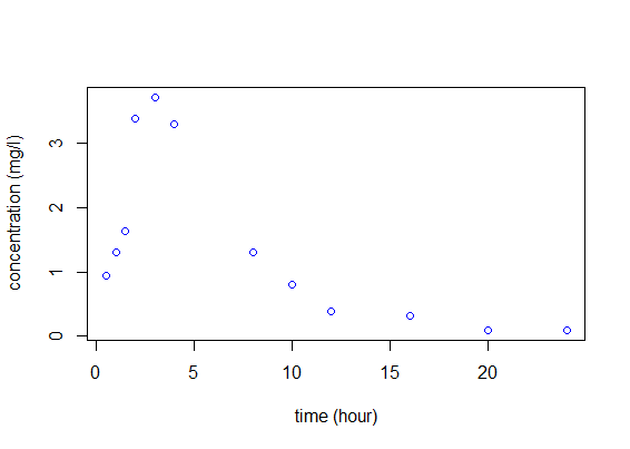
Let us consider a dose $D=50$ mg of a drug that is administrated orally to a patient at time 0. The concentrations of the drug are measured at times (0.5, 1.0, 1.5, 2.0, 3.0, 4.0, 8.0, 10.0, 12.0, 16.0, 20.0, 24.0).
pk1=read.table("example1_data.txt",header=T)
t=pk1$time
y=pk1$concentration
plot(t,y,xlab="time(hour)",ylab="concentration(mg/l)",col="blue")
|
There are two structural models that we can consider in order to evaluate the effects of such administration:
|
predc1=function(t,x){
A=50*x[1]/x[2]/(x[1]-x[3])
f=A*(exp(-x[3]*t)-exp(-x[1]*t))
}

predc2=function(t,x){
A=50/x[1]/x[2]/x[3]
ff=A*(1-exp(-x[3]*t))
ff[t>x[1]]=A*(1-exp(-x[3]*x[1]))*exp(-x[3]*(t[t>x[1]]-x[1]))
f=ff
}
|
We define then models ${\cal M}_1$ and ${\cal M}_2$ by assuming constant error models:
- \(\begin{align} {\cal M}_1 : \quad y_j & = & f_1(t_j ; \phi_1) + a_1\teps_j \\ {\cal M}_2 : \quad y_j & = & f_2(t_j ; \phi_2) + a_2\teps_j \end{align}\)
We can fit these two models to our data by computing $\hpsi_1=(\hphi_1,\hat{a}_1)$ and $\hpsi_2=(\hphi_2,\hat{a}_2)$, the MLEs of $\psi$ under models ${\cal M}_1$ and ${\cal M}_2$.
>>psi1 [1] 0.3240916 6.001204 0.3239337 0.4366948 >>psi2 [1] 3.203111 8.999746 0.229977 0.2555242 |
fmin1=function(x,y,t)
{f=predc1(t,x)
g=x[4]
e=sum( ((y-f)/g)^2 + log(g^2))}

fmin2=function(x,y,t)
{f=predc2(t,x)
g=x[4]
e=sum( ((y-f)/g)^2 + log(g^2))}

pk.nlm1=nlm(fmin1, c(0.3,6,0.2,1), y, t, hessian="true")
psi1=pk.nlm1$estimate

pk.nlm2=nlm(fmin2, c(3,10,0.2,4), y, t, hessian="true")
psi2=pk.nlm2$estimate
|
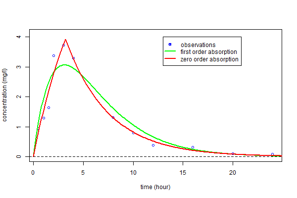
Therefore, the estimated parameters $\hphi_1$ and $\hphi_2$ can be used for computing predicted concentrations $\hat{f}_1(t)$ and $\hat{f}_2(t)$ under both models and for any time $t$.
We clearly see here that a much better fit is obtained with model ${\cal M}_2$, i.e. assuming a zero order absorption process.
tc=seq(from=0,to=25,by=0.1)
fc1=predc1(tc,phi1)
fc2=predc2(tc,phi2)
plot(t,y,ylim=c(0,4.1),xlab="time (hour)",ylab="concentration (mg/l)",col="blue")
lines(tc,fc1,type="l",col="green",lwd=2)
lines(tc,fc2,type="l",col="red",lwd=2)
abline(a=0,b=0,lty=2)
legend(13,4,c("observations","first order absorption","zero order absorption"),
       lty=c(-1,1,1),pch=c(1,-1,-1),lwd=2,col=c("blue","green","red"))
|
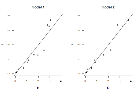
Another useful goodness of fit plot is obtained by displaying the observations $(y_j)$ versus the predictions $\hat{y}_j=f(t_j ; \hpsi)$ given by the model:
pk.nlm1=nlm(fmin1,c(0.3,6,0.2,1),y,t,hessian="true") f2=predc2(t,phi2) par(mfrow= c(1,2)) plot(f1,y,xlim=c(0,4),ylim=c(0,4),main="model 1") abline(a=0,b=1,lty=1) plot(f2,y,xlim=c(0,4),ylim=c(0,4),main="model 2") abline(a=0,b=1,lty=1) |
As we can see in the following paragraph, the Bayesian Information Criteria confirm the zero order absorption process should be selected.
>>bic1 [1] 24.10972 >>bic2 [1] 11.24769 |
deviance1=pk.nlm1$minimum + n*log(2*pi) bic1=deviance1+log(n)*length(psi1) deviance2=pk.nlm2$minimum + n*log(2*pi) bic2=deviance2+log(n)*length(psi2) |
We have only considered for the moment constant error models. Nevertheless, the graphic "observations vs predictions" seems to indicate that the amplitude of the residual errors increase with the prediction. We will then consider four different residual error models associated with the same structural model $f_2$.
|
fmin3=function(x,y,t)
{f=predc2(t,x)
g=x[4]*f
e=sum( ((y-f)/g)^2 + log(g^2))}

fmin4=function(x,y,t)
{f=predc2(t,x)
g=abs(x[4])+abs(x[5])*f
e=sum( ((y-f)/g)^2 + log(g^2))}

fmin5=function(x,y,t)
{f=predc2(t,x)
g=x[4]
e=sum( ((log(y)-log(f))/g)^2 + log(g^2))}
|
We can now compute $\hpsi_3=(\hphi_3,\hat{b}_3)$, $\hpsi_4=(\hphi_4,\hat{a}_4,,\hat{b}_4)$ and $\hpsi_5=(\hphi_5,\hat{a}_5)$, the MLEs of $\psi$ under models ${\cal M}_3$, ${\cal M}_4$ and ${\cal M}_5$.
>>psi3 [1] 2.642409 11.44113 0.1838779 0.2189221 >>psi4 [1] 2.890066 10.16836 0.2068221 0.02741416 0.1456332 >>psi5 [1] 2.710984 11.2744 0.188901 0.2310001 |
pk.nlm3=nlm(fmin3,c(phi2,0.1),y,t,hessian="true") psi3=pk.nlm3$estimate pk.nlm4=nlm(fmin4,c(phi2,1,0.1),y,t,hessian="true") psi4=pk.nlm4$estimate psi4[c(4,5)]=abs(psi4[c(4,5)]) pk.nlm5=nlm(fmin5, c(phi2,0.1),y,t,hessian="true") psi5=pk.nlm5$estimate |
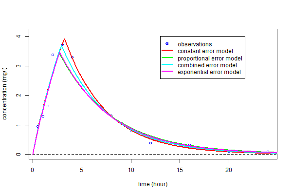
As you can see, the three predicted concentrations obtained with models ${\cal M}_3$, ${\cal M}_4$ and ${\cal M}_5$ are very similar
tc=seq(from=0,to=25,by=0.1)
fc1=predc1(tc,phi1)
fc2=predc2(tc,phi2)
plot(t,y,ylim=c(0,4.1),xlab="time (hour)",
     ylab="concentration (mg/l)",col = "blue")
lines(tc,fc1, type = "l", col = "green", lwd=2)
lines(tc,fc2, type = "l", col = "red", lwd=2)
abline(a=0,b=0,lty=2)
legend(13,4,c("observations","first order absorption","zero order absorption"),
       lty=c(-1,1,1), pch=c(1,-1,-1),lwd=2, col=c("blue","green","red"))
|
BIC confirms that a residual error model including a proportional component should be selected.
>> bic3 [1] 3.443607 >> bic4 [1] 3.475841 >> bic5 [1] 4.108521 |
deviance3=pk.nlm3$minimum + n*log(2*pi) bic3=deviance3 + log(n)*length(psi3) deviance4=pk.nlm4$minimum + n*log(2*pi) bic4=deviance4 + log(n)*length(psi4) deviance5=pk.nlm5$minimum + 2*sum(log(y)) + n*log(2*pi) bic5=deviance5 + log(n)*length(psi5) |
There is no obvious difference between these three error models. We will use the combined error model ${\cal M}_4$ in the following.
A 90% confidence interval for $\psi_4$ can derived from the Hessian matrix of the objective function.
>>ci4
            [,1]        [,2]
[1,]  2.22576690  3.55436561
[2,]  7.93442421 12.40228967
[3,]  0.16628224  0.24736196
[4,] -0.02444571  0.07927403
[5,]  0.04119983  0.25006660
|
alpha=0.9 df=n-length(phi4) I4=pk.nlm4$hessian/2 H4=solve(I4) s4=sqrt(diag(H4)*n/df) delta4=s4*qt(0.5+alpha/2,df) ci4=matrix(c(psi4-delta4,psi4+delta4),ncol=2) |
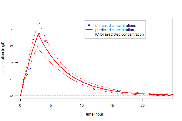
as well as a confidence interval for $f_4(t)$ using the Central Limit Theorem
nlpredci=function(phi,f,H)
{dphi=length(phi)
nf=length(f)
H=H*n/(n-dphi)
S=H[seq(1,dphi),seq(1,dphi)]
G=matrix(nrow=nf,ncol=dphi)
for (k in seq(1,dphi)) {
   dk=phi[k]*(1e-5)
   phid=phi
   phid[k]=phi[k] + dk
   fd=predc2(tc,phid)
   G[,k]=(f-fd)/dk }
M=rowSums((G%*%S)*G)
deltaf=sqrt(M)*qt(0.5+alpha/2,df)}

deltafc4=nlpredci(phi4,fc4,H4)

par(mfrow= c(1,1))
plot(t,y,ylim=c(0,4.5),xlab="time (hour)",ylab="concentration (mg/l)",col = "blue")
lines(tc,fc4, type = "l", col = "red", lwd=2)
lines(tc,fc4-deltafc4, type = "l", col = "red", lwd=1, lty=3)
lines(tc,fc4+deltafc4, type = "l", col = "red", lwd=1, lty=3)
abline(a=0,b=0,lty=2)
legend(10.5,4.5,c("observed concentrations","predicted concentration","IC for predicted concentration"),
       lty=c(-1,1,3), pch=c(1,-1,-1), lwd=c(2,2,1), col=c("blue","red","red"))
|
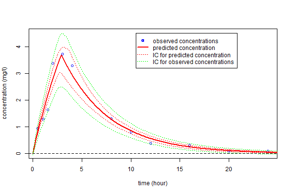
Alternatively, prediction intervals for $\hpsi_4$, $\hat{f}_4(t;\hpsi_4)$ and new observations at any time can be estimated by Monte-Carlo
>>ci4s
             [,1]        [,2]
[1,] 2.412131e+00  3.54008925
[2,] 8.554283e+00 11.89304332
[3,] 1.829453e-01  0.23922393
[4,] 1.558052e-08  0.08006378
[5,] 1.233954e-02  0.19552977
|
f=predc2(t,phi4)
a4=psi4[4]
b4=psi4[5]
g=a4+b4*f
dpsi=length(psi4)
nc=length(tc)
N=1000
qalpha=c(0.5 - alpha/2,0.5 + alpha/2)
PSI=matrix(nrow=N,ncol=dpsi)
FC=matrix(nrow=N,ncol=nc)
Y=matrix(nrow=N,ncol=nc)
for (k in seq(1,N)) {
   eps=rnorm(n)
   ys=f+g*eps
   pk.nlm=nlm(fmin4, psi4, ys, t)
   psie=pk.nlm$estimate
   psie[c(4,5)]=abs(psie[c(4,5)])
   PSI[k,]=psie
   fce=predc2(tc,psie[c(1,2,3)])
   FC[k,]=fce
   gce=a4+b4*fce
   Y[k,]=fce + gce*rnorm(1)
}

ci4s=matrix(nrow=dpsi,ncol=2)
for (k in seq(1,dpsi)){
   ci4s[k,]=quantile(PSI[,k],qalpha,names=FALSE)}

cifc4s=matrix(nrow=nc,ncol=2)
for (k in seq(1,nc)){
   cifc4s[k,]=quantile(FC[,k],qalpha,names=FALSE)}

ciy4s=matrix(nrow=nc,ncol=2)
for (k in seq(1,nc)){
   ciy4s[k,]=quantile(Y[,k],qalpha,names=FALSE)}
par(mfrow= c(1,1))
plot(t,y,ylim=c(0,4.5),xlab="time (hour)",ylab="concentration (mg/l)",col = "blue")
lines(tc,fc4, type = "l", col = "red", lwd=2)
lines(tc,cifc4s[,1], type = "l", col = "red", lwd=1, lty=3)
lines(tc,cifc4s[,2], type = "l", col = "red", lwd=1, lty=3)
lines(tc,ciy4s[,1], type = "l", col = "green", lwd=1, lty=3)
lines(tc,ciy4s[,2], type = "l", col = "green", lwd=1, lty=3)
abline(a=0,b=0,lty=2)
legend(10.5,4.5,c("observed concentrations","predicted concentration","IC for predicted concentration",
       "IC for observed concentrations"),lty=c(-1,1,3,3), pch=c(1,-1,-1,-1), lwd=c(2,2,1,1),
       col=c("blue","red","red","green"))
|
