Model evaluation
Contents
Introduction
Defining the expression "model evaluation" is a harder task than it may appear at first glance. Intuitively, it would seem to suggest evaluating the performance of a model based on the observed data, the same data that was used to build the model. Fair enough, but what then do we mean by the "performance" of a model?
Do we mean the ability of the model to characterize and explain the phenomena being studied, in which case the goal is to use the model to understand the phenomena? Or do we mean the model's predictive performance when the model is used to predict the phenomena's behavior, either in the future or under new experimental conditions?
What is comes down to is this: do we want to use the model to understand or to predict? This is the key question to ask before even starting to think about what tools to use and tasks to execute.
Here, we will be for the most part focused on the ability of a model to explain the phenomena and data. Therefore, the first goal will be to check whether the data are in agreement with the model, and vice versa. In this process, model diagnostics can be used to eliminate model candidates that do not seem capable of reproducing the observed data. As is the usual case in statistics, it is not because a model has not been rejected that it is necessarily the "true" one. All that we can say is that the experimental data does not allow us to reject this model. It is merely one of perhaps many models that cannot be rejected. Indeed, we can usually find several models that get past this first diagnostic step and are therefore not rejected.
What to do, then, when several possible models are retained? Well, we can try to select the "best" one (or best ones if no leader distinguishes itself from the rest). This means developing a model selection process which allows us to compare the models to each other. Compare models? But with what criteria?
In a purely explanatory context, Occam's razor is a useful parsimony principle which states that among competing hypotheses, the one with the fewest assumptions should be selected. In a modeling context, this means that among valid competing models, the most simple one should be selected.
Model diagnostic tools are for the most part graphical or visual: we "see" when something is not right between a chosen model and the data it is hypothesized to describe. Model selection tools, on the other hand, are analytical: we calculate the value of some criteria that allows us to compare the models with each other. However, it is absolutely critical to keep in mind the limits of these tools. These are not decision-making tools. It is not a $p$-value or some information criteria that can automatically decide which model to choose. It is always the modeler who must have the last word! This person uses the model diagnostic and selection tools in order to guide their decision, but at the end, it is they that must make the final decision. There is nothing more dangerous that rules applied without thinking and arbitrary cut-off values used blindly without reflection.
Here, we will not look model selection techniques based on the various models' predictive performances. One such approach consists of splitting the data into three sets: a learning set is used for fitting the model, a validation set for choosing between models and a test set to assess the quality of the predictions made by the chosen model.
Very few model diagnostic and selection tools exist for mixed-effects models. One of the most complete is Xpose, an R-based model-building aid for population analysis using NONMEM that facilitates model diagnostics, candidate covariate identification and model comparison. Here we will use $\monolix$ and illustrate these techniques with the example used previously for model exploration and parameter estimation.
Model diagnostics
Model diagnostics and statistical tests
Suppose first that a model has been entirely defined by the modeler, and that its parameters have either been chosen or estimated. What we call the "model" is therefore a joint probability distribution along with some parameter values.
Note ${\cal M}_0$ the model we wish to evaluate. We place ourselves in the framework of statistical testing, and would like to perform the following hypothesis test:
"Passing" the test does not mean that we accept $H_0$ but rather that we do not reject it. We will use the same point of view for model diagnostics whereby we eliminate model candidates that do not seem capable of reproducing the observed data, i.e., models for which we conclude that ${\cal M}\neq{\cal M}_0$.
To put into practice such a statistical test, we usually construct a test statistic $T(\by)$ which is a function of the observations and for which we are able to calculate a distribution under the null hypothesis $H_0$.
For a given significance level $\alpha$, we then define a rejection region $R_\alpha$ such that:
Thus, $\alpha$ is the probability of incorrectly rejecting the null hypothesis $H_0$.
The difficulty in creating and using such tests comes from two main things:
- We need to be capable of calculating the distribution of the test statistic $T(\by)$ under $H_0$ in order to carefully track the significance level, i.e., ensure that the probability of incorrectly rejecting $H_0$ is indeed $\alpha$.
- Being able to control the type I error $\alpha$ is of no interest if the test has low power, i.e., if the probability of correctly rejecting $H_0$ is low.
In the present context, the first point is clearly a problem. Due to the complexity of the models we are interested in, it is impossible to analytically calculate the distribution of a function of the observations, even for something as simple as the empirical mean $\overline{\by}=\sum_{i,j}y_{ij}/\sum_i{n_i}$.
Using limit theorems to approximate such distributions is also more or less hopeless. Perhaps the most powerful, general and precise solution we have available to us is Monte Carlo simulation:
- Generate independent values $\by^{(1)}, \by^{(2)}, \ldots , \by^{(L)}$ under the model ${\cal M}_0$ using the same design and covariates as in the original data.
- Calculate the $L$ statistics $T(\by^{(1)}), T(\by^{(2)}), \ldots , T(\by^{(L)})$.
- Estimate the distribution of $T(\by)$ under ${\cal M}_0$ with the empirical distribution of the $T(\by^{(\ell)})$.
The estimation error essentially depends on the number $L$ of simulated data sets. We must therefore choose $L$ large enough so that this error is negligible.
This solves part of the problem. But it remains hard to define a rejection region $R_\alpha$ if the test statistic is multidimensional. We can of course calculate relevant prediction intervals for each component of $T(\by)$ individually, but this does not really help us to define a real multidimensional rejection region.
Consequently, diagnostics methods are essentially visual: we compare the observed statistic $T(\by)$ with the expected distribution under ${\cal M}_0$ by graphically displaying (for example) 90% or 95% prediction intervals for each component of $T(\by)$.
The second point is also delicate because we need to decide what ${\cal M}\neq{\cal M}_0$ means, i.e., $H_0$ being false. Does it mean that the structural model is misspecified? Or the distribution of the random effects, the residual error model, the covariate model? There are so many ways in which a model can be misspecified that we cannot realistically expect to be able to create one unique statistic sufficiently powerful to detect all of these at once. We therefore prefer to construct several different test statistics, i.e., several graphical diagnostics tools, each good at dealing with one particular type of misspecification. It is then the combination of all these tools that will make up our test; we can fairly reasonably hope that a misspecified model will not succeed in passing through this filter.
Diagnostic plots using individual parameters
Diagnostic plots constructed using only the observations are useful for looking at the distribution $\qy$ of the observations, but do not help with testing hypotheses made on the non-observed individual parameters (about the distribution, covariate model, etc.).
One possible solution is to estimate the individual parameters (using for example the conditional mode) and then use these estimates to create new diagnostic tools. This strategy is only useful when the individual parameters have been estimated well.
If instead the data does not contain enough information to estimate certain individual parameters well, the individual estimates are all shrunk towards the same (population) value; this is the mode (resp. mean) of the population distribution of the parameter if we use the conditional mode (resp. conditional mean). For a parameter $\psi_i$ which is a function of a random effect $\eta_i$, we can quantify this phenomena by defining the so-called $\eta$-shrinkage as
where $\hat{\eta}_i$ is an estimate of $\eta_i$ (the conditional mode, conditional mean, etc.).
This shrinkage phenomenon is simple to understand because the conditional distribution $\qcetaiyi$ of $\eta_i$ is defined by the product $\pmacro(y_i|\eta_i)\pmacro(\eta_i)$. Saying that the observations $y_i$ provides little information about $\eta_i$ means that the conditional distribution of $y_i$ has a reduced importance in the construction of $\qcetaiyi$. The mode (resp. mean) of $\qcetaiyi$ will therefore be close to 0 which is both the mode and mean of $\qetai$. The result is a high level of shrinkage (close to 1) whenever $\var{\hat{\eta}_i}\ll\var{\eta_i}$.
Estimates of the $\psi_i$ are therefore biased because they do not correctly reflect the marginal distribution $\qpsii$ (in particular, their variance is much less). A particularly effective solution is to simulate the individual parameters $\psi_i$ with the conditional distribution $\qcpsiiyi$ rather than taking the mode. The resulting estimator is unbiased in the following sense:
This relationship is a fundamental one when considering inverse problems, incomplete data models, mixed-effects models, etc. So what does it imply exactly? Well, if we randomly draw a vector $y_i$ of observations for an individual in a population and then generate a vector $\psi_i$ using the conditional distribution $\qcpsiiyi$, then the distribution of $\psi_i$ is the population distribution $\qpsii$. In other words, even if each $\psi_i$ is simulated using its own conditional distribution, the fact of pooling them allows us to look at them as if they were a sample from $\qpsii$, i.e., the marginal distribution $\qpsii$ is a mixture of conditional distributions $\qcpsiiyi$.
The procedure is therefore as follows: we generate several values from each conditional distribution $\qcpsiiyi$ using the Metropolis-Hastings algorithm, and use them in addition to the observations in order to build various diagnostic plots.
An example
We are going to use the same model used for model exploration in the Visualization section and parameter estimation in the Maximum likelihood estimation of the population parameters chapter.
The structural model that defines the concentration in the central compartment and the hazard function for the events (hemorrhaging) is
The statistical model assumes that $ka_i$ and $V_i$ are log-normally distributed, $Cl_i$ normal, $h0_i$ probit-normal and $\gamma$ logit-normal. No covariates are used in this model. Lastly, we suppose a constant residual error model. Now we are going to review several different diagnostic plots and look at the conclusions that can be made using them.
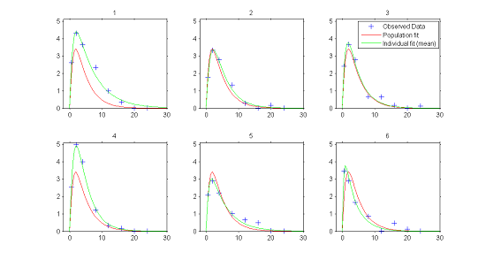
1) Individual fits.
In the continuous data model $y_{ij}=f(t_{ij};\psi_i) + f(t_{ij};\psi_i)\teps_{ij}$, estimation of the population parameters $\psi_{\rm pop}$ and individual parameters $\psi_{i}$ allows us to compute for each individual:
- $f(t ; \hat{\psi}_{\rm pop})$, the predicted profile given by the estimated population model
- $f(t ; \hat{\psi}_{i})$, the predicted profile given by the estimated individual model.
The figure plotting for each individual the two curves for the predicted concentration shows evidence of inter-individual variability in the kinetics, and furthermore does not allow us to reject the proposed PK model since the fits seem acceptable.
|
|
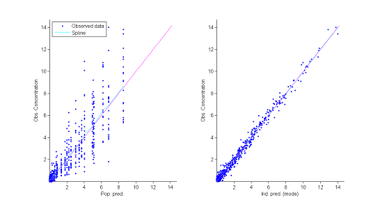
2) Observations vs predictions.
The population and individual models also allow us to calculate for each individual predictions at the observation times $f(t_{ij} ; \hat{\psi}_{\rm pop})$ and $f(t_{ij} ; \hat{\psi}_{i})$.
The figure showing observations vs individuals reveals no obvious misspecification. In particular it does not allow us to reject the constant residual error model.
|
|
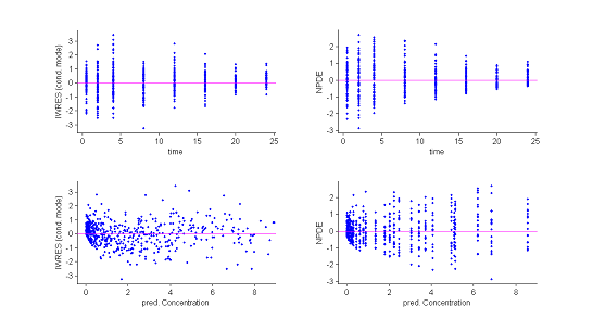
3) Residuals.
Several types of residuals can be defined: population weighted residuals $({\rm PWRES}_{ij})$, individual weighted residuals $({\rm IWRES}_{ij})$, normalised prediction distribution errors $({\rm NPDE}_{ij})$, etc. The first two are defined by:
where $\hat{\mathbb{E}}(y_{ij})$ and $\hat{\rm std}(y_{ij})$ are the mean and variance of $y_{ij}$ estimated by Monte Carlo. ${\rm NPDE}_{ij}$ is a nonparametric version of ${\rm PWRES}_{ij}$, based on a rank statistic. See npde for more details.
Statistics useful for summarizing the residuals are the 10%, 50% (median) and 90% quantiles. The procedure described earlier for estimating prediction intervals of these quantiles using Monte Carlo can again be used.
Both the individual residuals and the NPDEs suggest that the model is misspecified. Indeed, under ${\cal M}_0$ residuals are expected to behave as i.i.d. ${\cal N}(0,1)$ random variables, which is clearly not the case here. It is nevertheless difficult to identify the reasons for this misspecification using only these figures.
|
|
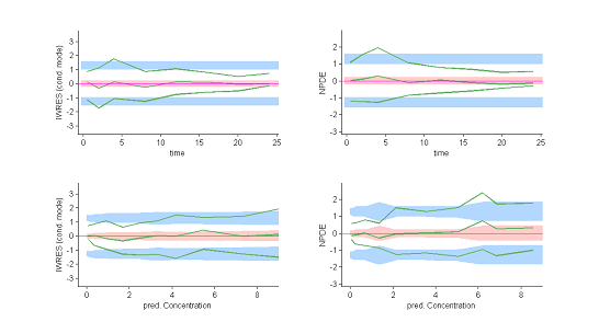
These plots show at each observation time the order 10%, 50% and 90% quantiles of the IWRES and NPDE.
The 90% prediction intervals are also displayed. These plots are more informative than the original residual plots. We can now reasonably conclude that the behavior of the three quantiles is not the one expected under ${\cal M}_0$. In particular, a proportional component in the residual error model appears not to have been taken into account. |
|
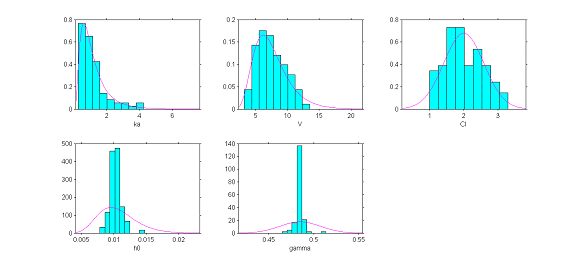
4) The distributions of the individual parameters.
The hypotheses we have made about the distributions of the individual parameters can be tested by visually comparing the pdf of the pre-selected distribution of each parameter with the empirical distribution of that parameter. We are going to see that using the estimated individual parameters does not allow us to construct a pertinent diagnostic plot, and that we must rather use parameters simulated with the conditional distribution $\qcpsiiyi$ for each individual.
The plots show for each model parameter the pdf obtained from the estimated parameters and the empirical distribution, shown as a histogram, of the estimated individual parameters (here the estimated parameters are the modes of the conditional distributions).
|
|
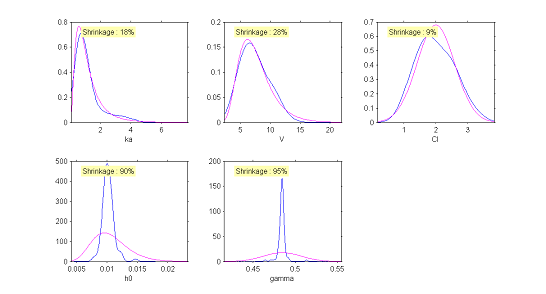
Instead of histograms, $\monolix$ can also display the empirical distribution of a continuous variable using nonparametric density estimation. This is a better way to represent continuous distributions than a histogram.
|
|
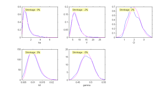
The simulated individual parameters now allow us to construct a diagnostic tool for the distributions of the individual parameters. Only the distribution of the clearance $Cl$ would appear to be rejected. Though the model had supposed a normal distribution, the simulated parameters seem to suggest an asymmetric distribution. This diagnostic plot leads us to think about testing the hypothesis of a log-normal distribution for $Cl$.
|
|
5) Covariate model.
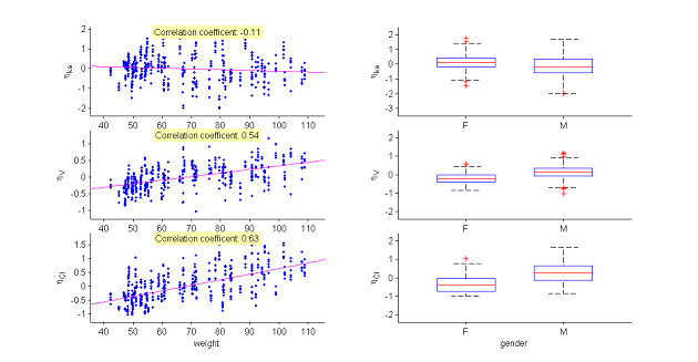
The model assumes that for a given individual parameter $\psi_i$, there exists a function $h$ such that $h(\psi_i) = h(\psi_{\rm pop}) + \eta_i$, where the random effects are i.i.d. Gaussian variables. We can then graphically display the random effects simulated with the conditional distributions as a function of the various covariates in order to see whether this hypothesis is valid.
These plots clearly show that the simulated random effects for $V$ and $Cl$ are correlated with the weight and have different distributions depending on gender. The assumption that volume $V$ and clearance $Cl$ are independent of weight should be rejected. The statistical model also needs to take into account the fact that both predicted volume and clearance increase with weight.
|
|
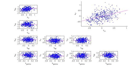
6) The correlation model. The model assumes that for a given individual, the random effects associated with the each individual parameter are independent. We can plot each pair of random effects simulated with the conditional distributions against each other to see if this hypothesis is valid.
The various point clouds show no correlation between random effects except for $(\eta_V,\eta_{Cl})$ and perhaps $(\eta_{ka},\eta_V)$.
|
|
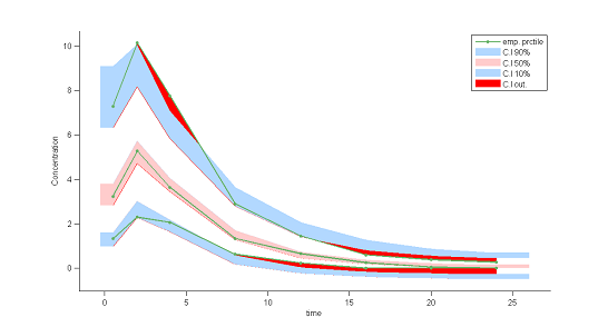
7) Visual predictive checks.
A VPC is a diagnostic tool well suited to continuous data. It allows us to summarize in the same figure the structural and statistical models. The VPC shown uses the order 10%, 50% and 90% for the observations after having regrouped them into bins for successive intervals. Then, prediction intervals for these quantiles under ${\cal M}_0$ are estimated using Monte Carlo.
To make it easier to interpret VPCs, we represent in red the zones where the observed quantiles are outside the prediction intervals. Here, the structural model seems to be ok, but the statistical model exhibits some incoherencies. In particular, the three quantiles obtained using the observations appear much closer together than the model ${\cal M}_0$ would suggest. This adds weight to the suggestion that a proportional component should be added to the error model.
|
|
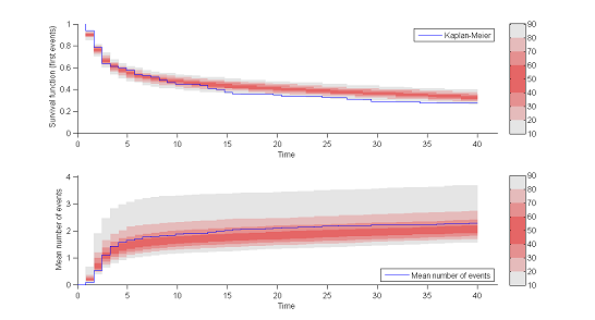
8) Kaplan Meier plots.
Special diagnostic plots need to be defined for non-continuous observations. We can for survival (time-to-event) data use Kaplan Meier plots (for the first event) as a statistic, and/or the average cumulated number of events per individual (i.e., the mean number of observed events before time $t$). The prediction intervals for these statistics can be estimated by Monte Carlo.
The shapes of the curves seem correct. The model appears to slightly overestimate the survival function after the 15 hr mark, but it is difficult at this point to decide whether this comes from the time-to-event model itself, the statistical model or the model for the concentration.
|
|
This new model can be easily implemented in $\monolix$. Population parameters and individual parameters are then estimated anew and new diagnostic plots drawn. A few of these are displayed below and clearly show that the new model is better than the previous one, and can likely be retained as a candidate model.

Model selection
Statistical tools for model selection
Statistical tools for model selection include information criteria (AIC and BIC) and hypothesis tests such as the Wald test and likelihood ratio test (LRT).
The Akaike Information Criteria (AIC) and the Bayesian information Criteria (BIC) are defined by
where $P$ is the total number of parameters to be estimated and $N$ the number of subjects. The models being compared using AIC or BIC need not be nested, unlike the case when models are being compared using an F-test or likelihood ratio test.
The observed log-likelihood ${\llike}(\theta;\by) = \log(\py(\by;\theta))$ cannot be computed in closed form for nonlinear mixed-effects models. It can be estimated by Monte Carlo using the importance sampling algorithm described in the Estimation of the log-likelihood section.
When comparing two nested models ${\cal M}_0$ and ${\cal M}_1$ with dimensions $P_0$ and $P_1$ (with $P_1>P_0$), the likelihood ratio test (LRT) uses the test statistic
where $\hthetag_0$ and $\hthetag_1$ are the MLE of $\theta$ under ${\cal M}_0$ and ${\cal M}_1$.
Depending on the hypotheses, the limit distribution of $LRT$ is either a $\chi ^2$ distribution or a mixture of a $\chi^2$ distribution and a Dirac $\delta$ distribution. For example:
-
- Testing whether some fixed effects are null and assuming the same covariance structure for the random effects implies that
- Testing whether some correlations in the covariance matrix $\IIV$ are null and assuming the same covariate model implies that
- Testing whether the variance of one of the random effects is zero and assuming the same covariate model implies that
Statistical tests, as is the case for BIC, help us decide whether the difference between two models is statistically significant.
Suppose that we want to test whether a fixed model parameter $\beta$ is null:
We construct a statistical test $T$ for which the distribution under $H_0$ allows us to calculate a $p$-value, i.e., the probability that $T$ is at least as big as the value observed under $H_0$. A small $p$-value leads us to reject $H_0$ with high confidence. It is usual to use the arbitrary cutoff of 5% to make this decision: we frequently read statements such as "a decrease in the objective function of a least 3.84 was required to identify a signifiant covariate". In the same way we could select models based on their BIC values under $H_0$ and $H_1$ by providing an arbitrary decision rule. It is sometimes suggested to choose $H_1$ if the difference $BIC_{H_1} -BIC_{H_0}$ is inferior to a certain arbitrary cutoff.
These approaches seem to simplify the modeler's life because they provide decision rules that can be applied systematically without thinking and thus justify decisions. But a rule, whatever it is, should never stop us asking why we are applying it and whether it is applicable in the present case. Remember that even a very small difference will be statistically significant if the sample size is large enough. The question is thus not to know whether a difference is statistically significant, but whether it is physically or biologically significant. We must therefore look carefully at the size of an effect and its real impact, both for understanding the model and for understanding its impact on the model's predictive capacities.
An example
We are going to continue using our joint model for concentration data and hemorrhaging events. The structural model is chosen to be the one used earlier for the diagnostic tests. We would now like to compare several statistical models:
${\cal M}_1$: all the individual parameters are log-normally distributed, there is no correlation between individual parameters, the residual error model is a combined one ($y=f+(a+b*f)*\teps$), both $\log(V)$ and $\log(Cl)$ are linear functions of $\log({\rm weight})$.
${\cal M}_2$: model ${\cal M}_1$, assuming that $\log(V_i)$ and $\log(Cl_i)$ are linearly correlated.
${\cal M}_3$: model ${\cal M}_2$, assuming that $\gamma_i=\gamma_{\rm pop}$ (i.e., $\omega_\gamma = 0$).
${\cal M}_4$: model ${\cal M}_2$, assuming that $Cl$ is not a function of the weight.
The results for these four models are as follows:
| Model | $-2\times {\llike}$ | BIC |
|---|---|---|
| ${\cal M}_1$ | 1390 | 1451 |
| ${\cal M}_2$ | 1370 | 1436 |
| ${\cal M}_3$ | 1370 | 1432 |
| ${\cal M}_4$ | 1446 | 1477 |
Clearly models ${\cal M}_2$ and ${\cal M}_3$ are the best in terms of BIC. We can therefore envisage selecting a model that includes both a correlation between $\log(V)$ and $\log(Cl)$ and that supposes that the volume $V$ is a function of the weight.
Rather than a purely statistical criteria (LRT or BIC) it is particularly the estimated value of the standard deviation of $\gamma$ ($\hat{\omega}_\gamma = 0.002$) under the model ${\cal M}_2$ that would lead us to conclude that the inter-individual variability of $\gamma$ is negligible.
It is also important to try and evaluate the impact that a bad decision could have. Retaining $\hat{\omega}_\gamma = 0.002$ would have little impact on predictions because $\gamma_i$ is log-normally distributed, representing a variability of around 0.2%. Models ${\cal M}_2$ and ${\cal M}_3$ are thus practically identical and there is no particular advantage of selecting one over the other.
Bibliography
Akaike, H. - Information measures and model selection
- Bulletin of the International Statistical Institute 50(1):277-291,1983
- BibtexAuthor : Akaike, H.
Title : Information measures and model selection
In : Bulletin of the International Statistical Institute -
Address :
Date : 1983
Arlot, S., Celisse, A. - A survey of cross-validation procedures for model selection
- Statistics Surveys 4:40 - 79,2010
- BibtexAuthor : Arlot, S., Celisse, A.
Title : A survey of cross-validation procedures for model selection
In : Statistics Surveys -
Address :
Date : 2010
Berger, J.O., Pericchi, L.R. - The intrinsic Bayes factor for model selection and prediction
- Journal of the American Statistical Association 91(433):109-122,1996
- BibtexAuthor : Berger, J.O., Pericchi, L.R.
Title : The intrinsic Bayes factor for model selection and prediction
In : Journal of the American Statistical Association -
Address :
Date : 1996
Bergstrand, M., Hooker, A.C., Wallin, J.E., Karlsson, M.O. - Prediction-corrected visual predictive checks for diagnosing nonlinear mixed-effects models
- The AAPS journal 13(2):143-151,2011
- BibtexAuthor : Bergstrand, M., Hooker, A.C., Wallin, J.E., Karlsson, M.O.
Title : Prediction-corrected visual predictive checks for diagnosing nonlinear mixed-effects models
In : The AAPS journal -
Address :
Date : 2011
Burnham, K.P., Anderson, D.R. - Model selection and multi-model inference: a practical information-theoretic approach
- Springer Verlag,2002
- BibtexAuthor : Burnham, K.P., Anderson, D.R.
Title : Model selection and multi-model inference: a practical information-theoretic approach
In : -
Address :
Date : 2002
Comets,E., Brendel,K. - Model evaluation in nonlinear mixed effect models, with applications to pharmacokinetics
- Journal de la Société Française de Statistique 151(1):106-128,2010
- BibtexAuthor : Comets,E., Brendel,K.
Title : Model evaluation in nonlinear mixed effect models, with applications to pharmacokinetics
In : Journal de la Société Française de Statistique -
Address :
Date : 2010
Comets, E., Brendel, K., Mentré, F. - Computing normalised prediction distribution errors to evaluate nonlinear mixed-effect models: the npde add-on package for R
- Computer methods and programs in biomedicine 90(2):154-166,2008
- BibtexAuthor : Comets, E., Brendel, K., Mentré, F.
Title : Computing normalised prediction distribution errors to evaluate nonlinear mixed-effect models: the npde add-on package for R
In : Computer methods and programs in biomedicine -
Address :
Date : 2008
Hausman, J., McFadden, D. - Specification tests for the multinomial logit model
- Econometrica: Journal of the Econometric Society pp. 1219-1240,1984
- BibtexAuthor : Hausman, J., McFadden, D.
Title : Specification tests for the multinomial logit model
In : Econometrica: Journal of the Econometric Society -
Address :
Date : 1984
Hooker, A., Karlsson, M.O., Jonsson, E.N. - Model diagnostic using XPOSE
- http://xpose.sourceforge.net/generic\_chm/xpose.VPC.html
BibtexAuthor : Hooker, A., Karlsson, M.O., Jonsson, E.N.
Title : Model diagnostic using XPOSE
In : -
Address :
Date :
Karlsson, M.O., Holford, N. - A Tutorial on Visual Predictive Checks
- PAGE 2008 ,2008
- http://www.page-meeting.org/pdf\_assets/8694-Karlsson_Holford_VPC_Tutorial_hires.pdf
BibtexAuthor : Karlsson, M.O., Holford, N.
Title : A Tutorial on Visual Predictive Checks
In : PAGE 2008 -
Address :
Date : 2008
Lavielle, M., Bleakley, K. - Automatic data binning for improved visual diagnosis of pharmacometric models
- Journal of pharmacokinetics and pharmacodynamics 38(6):861-871,2011
- BibtexAuthor : Lavielle, M., Bleakley, K.
Title : Automatic data binning for improved visual diagnosis of pharmacometric models
In : Journal of pharmacokinetics and pharmacodynamics -
Address :
Date : 2011
Massart, P. - Concentration Inequalities and Model Selection, Ecole d’Eté de Probabilités de Saint-Flour XXXIII-2003 Lecture Notes in Mathematics 1896
Neyman, J., Pearson, E.S. - On the problem of the most efficient tests of statistical hypotheses
Schwarz, G. - Estimating the dimension of a model
- The annals of statistics 6(2):461-464,1978
- BibtexAuthor : Schwarz, G.
Title : Estimating the dimension of a model
In : The annals of statistics -
Address :
Date : 1978
Shimodaira, H., Hasegawa, M. - Multiple comparisons of log-likelihoods with applications to phylogenetic inference
- Molecular biology and evolution 16:1114-1116,1999
- BibtexAuthor : Shimodaira, H., Hasegawa, M.
Title : Multiple comparisons of log-likelihoods with applications to phylogenetic inference
In : Molecular biology and evolution -
Address :
Date : 1999
Vaida, F., Blanchard, S. - Conditional Akaike information for mixed-effects models
- Biometrika 92(2):351--370,2005
- BibtexAuthor : Vaida, F., Blanchard, S.
Title : Conditional Akaike information for mixed-effects models
In : Biometrika -
Address :
Date : 2005
Wald, A. - Tests of statistical hypotheses concerning several parameters when the number of observations is large
- Transactions of the American Mathematical Society 54(3):426-482,1943
- BibtexAuthor : Wald, A.
Title : Tests of statistical hypotheses concerning several parameters when the number of observations is large
In : Transactions of the American Mathematical Society -
Address :
Date : 1943
Wilks, S.S. - The large-sample distribution of the likelihood ratio for testing composite hypotheses
- The Annals of Mathematical Statistics 9(1):60-62,1938
- BibtexAuthor : Wilks, S.S.
Title : The large-sample distribution of the likelihood ratio for testing composite hypotheses
In : The Annals of Mathematical Statistics -
Address :
Date : 1938
Zhao, P., Yu, B. - On model selection consistency of Lasso
- The Journal of Machine Learning Research 7:2541-2563,2006
- BibtexAuthor : Zhao, P., Yu, B.
Title : On model selection consistency of Lasso
In : The Journal of Machine Learning Research -
Address :
Date : 2006
 |
 |