Description, representation and implementation of a model
Contents
Introduction
A "model" can be implemented in the real world if it can be programmed using software. To do this, we need a language that can be understood by the software. Before even arriving at this point, it is important to be very clear and systematic about what a model is and how we want to use it.
It is fundamental to distinguish between the description, representation and implementation of a model. Each of these three concepts uses a specific language.
| 1. First, we describe a model with words, i.e., a human language: | "The weight is a linear function of the height" |
| 2. Then we represent the model using a mathematical or schematic language: | \( W=a\,H + b \) |
| 3. Lastly, we implement the model via a language understood by the software: | WEIGHT = a*HEIGHT + b |
The representation of a model is not unique. The choice of the representation should be driven by the tasks to be executed: if the model is only used to perform computations, a system of equations contains all the information required. If properties of the model need to be tested (linearity, homoscedasticity, etc.), then they need to be represented via explicit definitions.
In the context of mixed-effects models, models that we want to implement can be decomposed into two components: the structural model and the statistical model. Both components have to be described, represented and implemented with precision.
Description, representation and implementation of the structural model
Let us now look in more detail at these three things.
Description of the structural model
The first step consists in describing a model with high precision, using terminology and vocabulary well-adapted to the application. For instance, let us consider a PK model that describes drug concentration as a function of time. We can describe the model with the sentence:
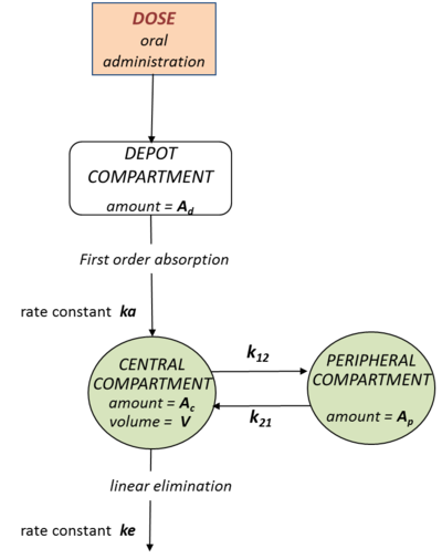
"The PK model is a two-compartment model with first-order absorption (from the depot compartment - the gut, to the central compartment - the bloodstream), linear transfers between the central and the peripheral compartment, and linear elimination from the central compartment".
Representation of the structural model
1. Using a diagram
This PK model can by represented by a diagram like the one shown the the following figure. Such diagrams offer both a descriptive and explicit representation (because the properties of the PK model are clearly shown).
2. Using mathematical equations
Alternatively, a mathematical representation can be used to translate the description of the model into a system of equations:
This representation allows us to calculate the amount of drug in each compartment at any point of time. On the other hand, this description of the model is implicit: even if a modeler is able to recognize the model described by the equations, i.e., to identify the processes of absorption, distribution and elimination, these are not explicitly represented like in the diagram.
Implementation of the structural model
1. Using macros
The $\mlxtran$ language allows us to implement the model represented in the previous diagram using a simple script and a system of macros:
As you can see, there is a one-to-one mapping between the diagram and the code: each element of the diagram (and therefore of the model) is implemented as a macro.
2. Using equations
Alternatively, implementation of the model using the mathematical representation requires entering the system of equations into $\mlxtran$. The syntax used should be as close as possible to the original mathematical language in order make development simple and the code easy to parse. Here is the $\mlxtran$ syntax in this case:
Which representation for which task?
It is fundamental to have the possibility of using several representations, and therefore several implementations, depending on the task at hand. One reason is that each kind of implementation has its pros and cons.
The use of equations has the big advantage of being able to represent any complex model. This is not possible when using macros, which are fixed in number by default. For instance, the PK macros in $\mlxtran$ allow us to code linear and nonlinear (Michaelis-Menten) elimination, but no macro exists that can combine the two types of elimination. In contrast, such processes can be easily input using equations:
- ddt_Ac= ka*Ad - k12*Ac + k21*Ap - k*Ac - Vm*Ac/(Km*V + Ac)
In a similar vein, models that are well-defined mathematically may be horribly complex to implement using equations, but easy using macros. This is true for instance for dynamical systems with source terms such as PK models with repeated oral doses and zero-order absorption. In that example, the absorption rate is a piecewise-constant function. It is not easy to code this model using equations, and not worth it when we can quickly use the $\mlxtran$ macro oral(Tk0), which completely characterizes the model for any dose design. The C++ code generated from an $\mlxtran$ script that uses this macro is the same as the one (that would be) generated by a script using a system of equations.
Description, representation and implementation of the statistical model
The statistical component of the model can be decomposed in two sub-models: a model that describes the variability of the parameters and a model that describes the variability of the observations. Each sub-model needs to be described, represented and implemented. Let us illustrate this approach with a very simple statistical model used for modeling the variability of a single individual parameter.
Description of the statistical model
In this example we want to describe the distribution of the volume in the population, using weight as a covariate. The first step consists of describing with extreme precision the statistical model that we want to use:
- Individuals in the population are mutually independent
- The volume is log-normally distributed
- The log-volume predicted by the model is a linear function of the log-weight
- The reference weight in the population is 70kg
- The variance of the log-volume is constant.
Representation of the statistical model
Since this model involves probability distributions, we will use a probabilistic model to represent it. Let $V_i$ and $w_i$ be the volume and weight of individual $i$. Statement 1 implies that only the conditional distribution $p(V_i | w_i)$ for individual $i$ needs to be represented. A probability distribution can be mathematically represented by a series of definitions and equations. This mathematical representation is not unique. We can use for instance any of these three representations:
\(\begin{eqnarray}
V_i &=& \Vpop \left(\displaystyle{ \frac{w_i}{70} }\right)^\beta \, e^{\eta_i} \quad \text{where} \quad \eta_i \sim {\cal N}(0, \omega^2)
\end{eqnarray}\)
|
(1) |
\(\begin{eqnarray}
\hat{V}_i &=& \Vpop \left(\displaystyle{ \frac{w_i}{70} }\right)^\beta \quad \text{and} \quad
\log(V_i) \sim {\cal N}(\log(\hat{V}_i) , \omega^2)
\end{eqnarray}\)
|
(2) |
\(\begin{eqnarray}
\tilde{w}_i& =& \log\left(\displaystyle{ \frac{w_i}{70} }\right) \quad \text{and} \quad \log(V_i) \sim {\cal N}(\log(\Vpop)+\beta \, \tilde{w}_i , \omega^2) .
\end{eqnarray}\)
|
(3) |
Here, $\omega$ is the standard deviation of the log-volume, $\Vpop$ is a reference value of volume in the population for a reference individual of 70kg and $\Vpop (w_i/70)^\beta$ the predicted volume for an individual with weight $w_i$.
These three representations combine equations and definitions. The equations allow us to define the variables via algebraic equations, while the definitions characterize the random variables via probability distributions.
Implementation of the statistical model
The implementation of such models with $\mlxtran$ allows the direct usage of the same definitions and equations with a language very close to the mathematical one. The model in (1) can be implemented in the following way:
The model in (2) can be implemented this way:
The model in (3) can be implemented like this:
Note that the linearity of the model is information that is explicitly entered.
Which representation for which task?
Representations (1), (2) and (3) provide three different mathematical representations of the same probabilistic model. This means that when any of them are written in text or on a slide, anyone with some basic knowledge in statistics and mathematics will be able to derive the same information from any of the representations.
However, if we want to use the model to perform tasks using specific software, the information passed to the software needs to be of a form that the software can understand with respect to each given task. It is not always true that any representation paired with any implementation can be used to perform any task. Let us illustrate this on our example for three basic tasks: simulation, likelihood computation and covariate model assessment.
Simulation. If we assume that the software we use is able to simulate normal random variables with any given mean and standard deviation, then any representation of the model can be used for simulation:
- Using (1), $\eta_i$ is first simulated as a normal random variable with mean 0 and variance $\omega^2$. Then the volume $V_i$ is calculated as a function of $\eta_i$.
In summary, what is required for simulation is the capacity to express the variable to be simulated as a function of some random variable that can be directly simulated by the software. In conclusion, any of the three $\mlxtran$ implementations proposed above can be used for simulation.
Likelihood computation. By definition, the likelihood of a set of parameter values given some continuous observed outcomes is equal to the probability distribution function (pdf) of those observed outcomes given those parameters. In other words, to derive the likelihood of $\theta=(\Vpop,\beta,\omega^2)$ requires computation of the pdf of $V_i$ or a certain function of it. Here, it is straightforward to derive the likelihood from the pdf of $V_i$, which is log-normally distributed:
\(\begin{eqnarray}
L_1(\theta ; V_1,\ldots,V_N) &=& \py(V_1,V_2,\ldots,V_N ;\theta) \\
& = & \prod_{i=1}^N \py( V_i ;\theta) \\
& = & \prod_{i=1}^N \displaystyle{ \frac{1}{\sqrt{2\pi \omega}V_i} } \exp\left\{-\displaystyle{ \frac{1}{2\omega} } \left( \log(V_i) - \log\left(\Vpop \left({w_i}/{70}\right)^\beta\right) \right)^2\right\} .
\end{eqnarray}\)
|
(4) |
It is also straightforward to derive the likelihood from the pdf of $\log(V_i)$, which is normally distributed:
\(\begin{eqnarray}
L_2(\theta ; \log(V_1),\ldots,\log(V_N)) &=& \py(\log(V_1),\ldots,\log(V_N) ;\theta) \\
& = & \prod_{i=1}^N \displaystyle{ \frac{1}{\sqrt{2\pi \omega} } }\exp\left\{-\frac{1}{2\omega} \left( \log(V_i) - \log\left(\Vpop \left({w_i}/{70}\right)^\beta\right) \right)^2 \right\} .
\end{eqnarray}\)
|
(5) |
These two likelihoods $L_1$ and $L_2$ are equal up to a constant $\prod_i V_i$. No matter what the definition of the likelihood is based on, it is nonetheless necessary to provide some information about the pdf of $V_i$ for computing the likelihood. In this very basic example, the minimal information about the model that needs to be passed to the software via code to be able to compute the likelihood is:
- The log-volume is normally distributed
- The mean of $\log(V_i)$ is $\log\left(\Vpop \left({w_i}/{70}\right)^\beta\right)$
- The standard deviation of $\log(V_i)$ is $\omega$.
Then, the likelihood can be easily computed if the software is able to compute a normal pdf for a given mean and standard deviation.
In our example, only the representations of the model given in (2) and (3) (and therefore versions 2 and 3 of the $\mlxtran$ implementation) can be used for computing the likelihood in closed form. Indeed, both representations explicitly describe the probability distribution of $\log(V_i)$ and provide all the required information. On the other hand, the representation given in (1) does not provide any explicit information about the distribution of $V_i$. Deriving the pdf of $V_i$ from (1) would therefore require an interpreter to "understand" the formula, and a tool that can perform symbolic computation.
Covariate model assessment. Our model hypothesizes a linear relationship between the log-weight and the log-volume.
To assess if this is valid or not, we might consider using some visual diagnostic check of the plot of the (predicted or simulated) log-volume against the log-weight, to see whether this linear relationship seems plausible or not. Specific statistical procedures can also be used for testing the linearity hypothesis.
Thus, both displaying an appropriate goodness of fit plot and using an appropriate statistical test require knowledge of the explicit relationship between the covariate and the parameter, i.e., the software needs to "know" this relationship. Neither of the representations of the model based on equations (1) and (2) explicitly spell out this relationship to the software. Of course, we can rewrite (2) as:
and clearly "see" that the predicted log-volume is a linear function of the log-weight. The issue is that, without a powerful interpreter, this information is not available to the software, so it cannot automatically run these tasks. Therefore, we must explicitly "tell" the software that the model is linear, as can be done with $\mlxtran$.
 |