Difference between revisions of "Overview"
Jump to navigation
Jump to search
m |
m |
||
| Line 2: | Line 2: | ||
Data: concentrations at times $0, 1, \ldots 15$, from 6 patients who received each 100 mg at time $t=0$ (bolus intravenous): | Data: concentrations at times $0, 1, \ldots 15$, from 6 patients who received each 100 mg at time $t=0$ (bolus intravenous): | ||
| − | [[Image:Intro1.png|center| | + | [[Image:Intro1.png|center|900px]] |
| Line 19: | Line 19: | ||
* Observed concentration at time $t_j$, $j=1, 2, \ldots, 15$: | * Observed concentration at time $t_j$, $j=1, 2, \ldots, 15$: | ||
| − | + | ||
| − | y_j = f(t_j ; V,k) + \varepsilon_j | + | |
| − | + | ||
| + | :: <div style="text-align: left;font-size: 15pt"><math> y_j = f(t_j ; V,k) + \varepsilon_j </math></div> | ||
| + | |||
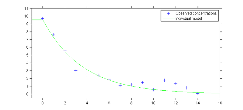
Observed concentrations from individual 1 and predicted concentration profile obtained with $V=10.5$ and $k=0.279$: | Observed concentrations from individual 1 and predicted concentration profile obtained with $V=10.5$ and $k=0.279$: | ||
| − | [[Image:Intro2.png|center| | + | [[Image:Intro2.png|center|800px]] |
Revision as of 15:23, 1 February 2013
Data: concentrations at times $0, 1, \ldots 15$, from 6 patients who received each 100 mg at time $t=0$ (bolus intravenous):
Goal of modelling: describe the variability of the data (structural, intra $\&$ inter variabilities) using a statistical model.
The classical individual approach derives a model for a unique individual.
- Predicted concentration at time $t$:
- \( f(t ; V,k) = \frac{D}{V} \ e^{-k \, t} \)
- Observed concentration at time $t_j$, $j=1, 2, \ldots, 15$:
- \( y_j = f(t_j ; V,k) + \varepsilon_j \)
Observed concentrations from individual 1 and predicted concentration profile obtained with $V=10.5$ and $k=0.279$:
