Difference between revisions of "Overview"
m |
m |
||
| Line 1: | Line 1: | ||
| + | |||
| + | |||
| + | In the following sections we introduce a formalism to describe the individual models and to calculate some useful information (confidence intervals, Fisher information Matrix, etc.) about the descriptors. The implementation of such formalism in a software and the corresponding results will be also illustrated. | ||
| + | |||
| + | Let us start our discussion with a couple of examples. | ||
| + | |||
| + | |||
| + | |||
Data: concentrations at times $0, 1, \ldots 15$, from 6 patients who received each 100 mg at time $t=0$ (bolus intravenous): | Data: concentrations at times $0, 1, \ldots 15$, from 6 patients who received each 100 mg at time $t=0$ (bolus intravenous): | ||
| − | {|cellpadding=" | + | {|cellpadding="0" cellspacing="0" |
| − | | style="width: 300px | + | | style="width: 300px" | |
[[File:Intro1.png]] | [[File:Intro1.png]] | ||
|} | |} | ||
Revision as of 17:00, 8 February 2013
In the following sections we introduce a formalism to describe the individual models and to calculate some useful information (confidence intervals, Fisher information Matrix, etc.) about the descriptors. The implementation of such formalism in a software and the corresponding results will be also illustrated.
Let us start our discussion with a couple of examples.
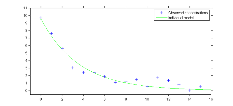
Data: concentrations at times $0, 1, \ldots 15$, from 6 patients who received each 100 mg at time $t=0$ (bolus intravenous):
Goal of modelling: describe the variability of the data (structural, intra $\&$ inter variabilities) using a statistical model.
The classical individual approach derives a model for a unique individual.
- Predicted concentration at time $t$:
- \( f(t ; V,k) = \frac{D}{V} \ e^{-k \, t} \)
- Observed concentration at time $t_j$, $j=1, 2, \ldots, 15$:
- \( y_j = f(t_j ; V,k) + \varepsilon_j \)
Observed concentrations from individual 1 and predicted concentration profile obtained with $V=10.5$ and $k=0.279$:
