Difference between revisions of "Introduction to PK modeling using MLXPlore - Part II"
m |
m (→Introduction) |
||
| (6 intermediate revisions by the same user not shown) | |||
| Line 1: | Line 1: | ||
== Introduction== | == Introduction== | ||
| − | We display here the amounts both in the central and depot compartments for the various PK models presented in [[ | + | We display here the amounts both in the central and depot compartments for the various PK models presented in the [[Introduction to PK modeling using MLXPlore - Part I | Part I]]. We also show the $\mlxtran$ code that was used for computing these two quantities. |
<br> | <br> | ||
| + | |||
== Absorption == | == Absorption == | ||
| Line 17: | Line 18: | ||
<div style="overflow-x:auto"> | <div style="overflow-x:auto"> | ||
{| cellpadding="10" cellspacing="10" | {| cellpadding="10" cellspacing="10" | ||
| − | |style="width:50%"| [[File:Absorption1b_script.png | + | |style="width:50%"| [[File:Absorption1b_script.png]] |
|style="width:50%"| | |style="width:50%"| | ||
| − | [[File:Absorption1b.png | + | [[File:Absorption1b.png]] |
|} </div> | |} </div> | ||
| Line 33: | Line 34: | ||
<div style="overflow-x:auto"> | <div style="overflow-x:auto"> | ||
{| cellpadding="10" cellspacing="10" | {| cellpadding="10" cellspacing="10" | ||
| − | |style="width:50%"| [[File:Absorption2b_script.png | + | |style="width:50%"| [[File:Absorption2b_script.png]] |
|style="width:50%"| | |style="width:50%"| | ||
| − | [[File:Absorption2b.png | + | [[File:Absorption2b.png]] |
|} </div> | |} </div> | ||
| Line 49: | Line 50: | ||
<div style="overflow-x:auto"> | <div style="overflow-x:auto"> | ||
{| cellpadding="10" cellspacing="10" | {| cellpadding="10" cellspacing="10" | ||
| − | |style="width:50%"| [[File:Absorption3b_script.png | + | |style="width:50%"| [[File:Absorption3b_script.png]] |
|style="width:50%"| | |style="width:50%"| | ||
| − | [[File:Absorption3b.png | + | [[File:Absorption3b.png]] |
|} </div> | |} </div> | ||
| Line 65: | Line 66: | ||
<div style="overflow-x:auto"> | <div style="overflow-x:auto"> | ||
{| cellpadding="10" cellspacing="10" | {| cellpadding="10" cellspacing="10" | ||
| − | |style="width:50%"| [[File:Absorption4b_script.png | + | |style="width:50%"| [[File:Absorption4b_script.png]] |
|style="width:50%"| | |style="width:50%"| | ||
| − | [[File:Absorption4b.png | + | [[File:Absorption4b.png]] |
|} </div> | |} </div> | ||
| Line 82: | Line 83: | ||
<div style="overflow-x:auto"> | <div style="overflow-x:auto"> | ||
{| cellpadding="10" cellspacing="10" | {| cellpadding="10" cellspacing="10" | ||
| − | |style="width:50%"| [[File:Absorption5b_script.png | + | |style="width:50%"| [[File:Absorption5b_script.png]] |
|style="width:50%"| | |style="width:50%"| | ||
| − | [[File:Absorption5b.png | + | [[File:Absorption5b.png]] |
|} </div> | |} </div> | ||
| Line 94: | Line 95: | ||
<span style="color:#993300">{{Verbatim|absorption6b_script: }}</span> we compute and display the amounts in the central and depot compartments for the various absorption models presented in the previous examples. | <span style="color:#993300">{{Verbatim|absorption6b_script: }}</span> we compute and display the amounts in the central and depot compartments for the various absorption models presented in the previous examples. | ||
| − | In the figure on the right side, | + | In the figure on the right side, abs1 is first-order absorption, abs2 is $\alpha$-order absorption, abs3 is saturated absorption, abs4 is zero-order absorption and abs5 is sequential zero-order/first-order absorption. |
<div style="overflow-x:auto"> | <div style="overflow-x:auto"> | ||
{| cellpadding="10" cellspacing="10" | {| cellpadding="10" cellspacing="10" | ||
| − | |style="width:50%"| [[File:Absorption6b_script.png | + | |style="width:50%"| [[File:Absorption6b_script.png]] |
|style="width:50%"| | |style="width:50%"| | ||
| − | [[File:Absorption6b.png | + | [[File:Absorption6b.png]] |
|} </div> | |} </div> | ||
| Line 108: | Line 109: | ||
{{Back | {{Back | ||
| − | |link | + | |link=Introduction to PK modeling using MLXPlore - Part I }} |
Latest revision as of 10:18, 29 May 2013
Contents
Introduction
We display here the amounts both in the central and depot compartments for the various PK models presented in the Part I. We also show the $\mlxtran$ code that was used for computing these two quantities.
Absorption
First-order and zero-order absorption
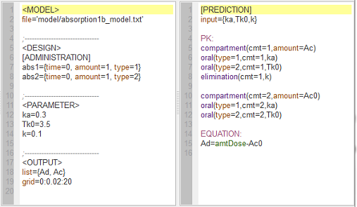
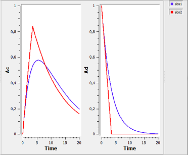
absorption1b_script: we compute and display both the amount $Ac$ in the central compartment (as before) and the amount Ad in the depot compartment when a single dose is administered at time $t=0$.
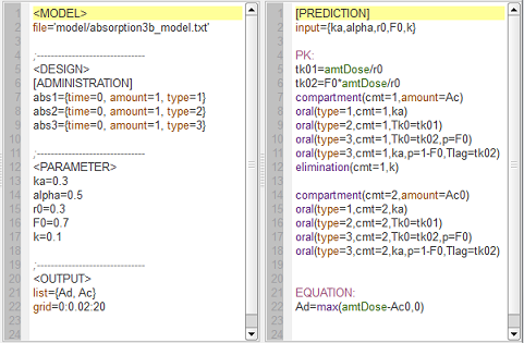
When PK macros are used for absorption, the amount in the depot can be computed by first creating another central compartment (cmt=2) which receives the same dose as the central compartment (cmt=1) with the same absorption processes, but without elimination. The amount in the depot is then the total dose administered minus the amount in the second central compartment.
Zero-order, first-order and $\alpha$-order absorption
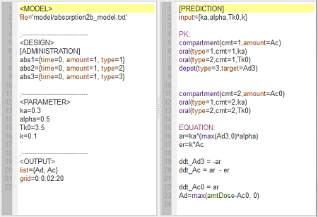
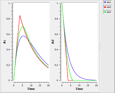
absorption2b_script: we compute and display the amounts in the central and depot compartments when the drug is transferred from the depot to the central compartment with a first-order, zero-order or $\alpha$-order absorption process.
Note $\dot{A}d(t) \, = \, -ka \, \times \, Ad^{\alpha}(t).$ Zero-order absorption is obtained with $\alpha=0$ and first-order absorption with $\alpha=1$. The blue, red and green curves are obtained respectively with first-order, zero-order and $\alpha$-order absorption processes.
First-order, zero-order and sequential zero-order/first-order absorption
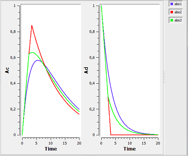
absorption3b_script: we compute and display the amounts in the central and depot compartments when the drug is transferred from the depot to the central compartment with a first-order, zero-order or sequential zero-order/first-order absorption process.
The blue, red and green curves are obtained respectively with first-order, zero-order and sequential zero-order/first-order absorption processes.
First-order and saturated absorption
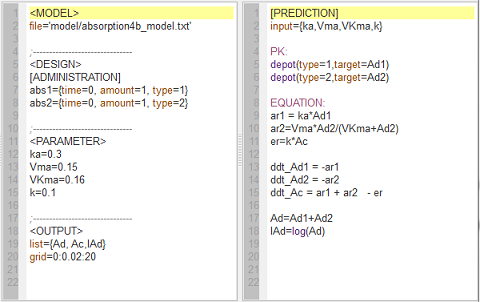
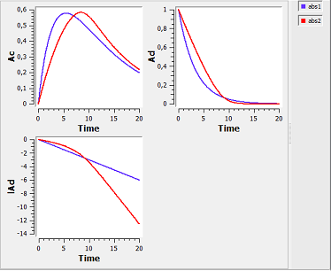
absorption4b_script: we compute and display the amounts in the central and depot compartments when the drug is transferred from the depot to the central compartment with a first-order or saturated (Michaelis-Mentens) absorption process.
The red curve is now for the saturated absorption process. The log plot ($lAd$ vs $Time$) shows that the log of the amount in the depot department $lAd$ decreases linearly for first-order absorption but not for saturated absorption.
Lag-time and transit compartments
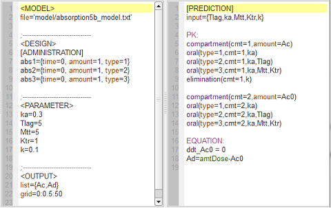
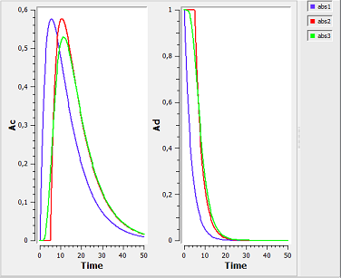
absorption5b_script: we compute and display the amounts in the central and depot compartments when a lag time or transit compartment model is used.
Here, the blue curves are for first-order absorption without lag-time, red curves for the lag-time model and green for the transit compartment model. The number of transit compartments is $Ntr=Mtt/Ktr$. When $Mtt=Tlag$, the transit compartment model compartment can be seen as a smooth version of the lag-time model. It converges to the lag-time model when the number of compartments increases (i.e., when the transfer rate constant $Ktr$ increases).
Summary
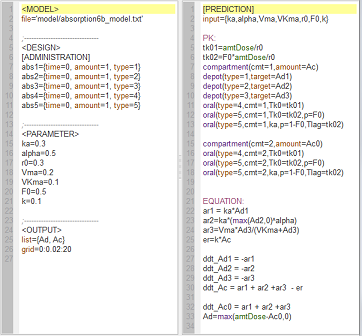
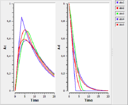
absorption6b_script: we compute and display the amounts in the central and depot compartments for the various absorption models presented in the previous examples.
In the figure on the right side, abs1 is first-order absorption, abs2 is $\alpha$-order absorption, abs3 is saturated absorption, abs4 is zero-order absorption and abs5 is sequential zero-order/first-order absorption.
All the projects shown in this session can be downloaded here: https://wiki.inria.fr/wikis/popix/images/c/c6/Pk_mlxplore.zip.
