Continuous data models
$ \newcommand{\pcyipsii}{p_{y_i|\psi_i}} \newcommand{\bpsi}{\boldsymbol{\psi}} \newcommand{\bu}{\boldsymbol{u}} \newcommand{\bx}{\boldsymbol{x}} \newcommand{\by}{\boldsymbol{y}} \newcommand{\hazard}{h} \newcommand{\prob}[1]{ \mathbb{P}\!\left(#1\right)} \newcommand{\probs}[2]{ \mathbb{P}_{#1}\!\left(#2\right)} \newcommand{\Rset}{\mbox{$\mathbb{R}$}} \newcommand{\Yr}{\mbox{$\mathcal{Y}$}} \newcommand{\teps}{\tilde{\varepsilon}} \newcommand{\std}[1]{\mbox{sd}\left(#1\right)} \newcommand{\esp}[1]{\mathbb{E}\left(#1\right)} $
Introduction
We focus in this section on the model for the observations $\by=(\by_i, \ 1\leq i \leq N)$, i.e., the conditional probability distributions $\{\pcyipsii(\by_i | \bpsi_i), \ 1\leq i \leq N\}$, where
- $N$ is the number of subjects.
- $\by_i = (y_{ij}, \ 1\leq j \leq n_i)$ are the $n_i$ observations for individual $i$. Here, $y_{ij}$ is the measurement made on individual $i$ at time $t_{ij}$.
- $\bpsi_i$ is the vector of individual parameters for subject $i$.
Remarks:
- We suppose that the model we will use to describe the observations is a function of regression variables $\bx_i = (x_{ij}, \ 1\leq j \leq n_i)$. Each $x_{ij}$ is made up of the time $t_{ij}$ and perhaps other variables that vary with time. For example, a pharmacokinetic model can depend on time and weight: $x_{ij} = (t_{ij},w_{ij})$ where $w_{ij}$ is the weight of individual $i$ at time $t_{ij}$, whereas a pharmacodynamic model can depend on time and concentration: $x_{ij} = (t_{ij},c_{ij})$.
- The model for individual $i$ can also depend on {\it input terms} $\bu_i$. For example, a pharmacokinetic model include the dose regimen administrated to the patients:
$\bu_i$ is made up of the dose(s) given to patient $i$, the time(s) of administration, and their type (IV bolus, infusion, oral, etc.). If the structural model is a dynamical system (e.g., defined by a system of ODEs), the input terms $(\bu_i)$ are also called source terms, see the Dynamical systems driven by ODEs chapter for more details.
In our framework, observations $\by$ are longitudinal. So, for a given individual $i$,
the model has to describe the change in $\by_i=(y_{ij})$ over time. To do this, we suppose that each observation $y_{ij}$ comes from a probability distribution, one that evolves with time. As we have decided to work with parametric models, we suppose that there exists a function $\lambda$ such that the distribution of $y_{ij}$ depends on $\lambda(t_{ij},\psi_i)$. Implicitly, this includes the time-varying variables $x_{ij}$ mentioned above.
The time-dependence in $\lambda$ helps us to describe the change with time of each $\by_i$, while the fact it depends on the vector of individual parameters $\psi_i$ helps us to describe the inter-individual variability in $\by_i$.
We will distinguish in the following between continuous data models, discrete data models (including categorical and count data) and time-to-event (or survival) models.
Here are some examples of these various types of data:
- Continuous data with a normal distribution:
- \( y_{ij} \sim {\cal N}\left(f(t_{ij},\psi_i),\, g^2(t_{ij},\psi_i)\right) \)
- Here, $\lambda(t_{ij},\psi_i)=\left(f(t_{ij},\psi_i),\,g(t_{ij},\psi_i)\right)$, where $f(t_{ij},\psi_i)$ is the mean and $g(t_{ij},\psi_i)$ the standard deviation of $y_{ij}$.
- Categorical data with a Bernoulli distribution:
- \( y_{ij} \sim {\cal B}\left(\lambda(t_{ij},\psi_i)\right) \)
- Here, $\lambda(t_{ij},\psi_i)$ is the probability that $y_{ij}$ takes the value 1.
- Count data with a Poisson distribution:
- \( y_{ij} \sim {\cal P}\left(\lambda(t_{ij},\psi_i)\right) \)
- Here, $\lambda(t_{ij},\psi_i)$ is the Poisson parameter, i.e., the expected value of $y_{ij}$.
- Time-to-event data:
- \( \begin{array}{rcl} \prob{y_{i} >t} &= & S( t,\psi_i) \\[6pt] - \displaystyle{\frac{d}{dt}} \log S(t,\psi_i) &= & \hazard(t,\psi_i) \end{array} \)
- Here, $\lambda(t,\psi_i) = \hazard(t,\psi_i)$ is known as the hazard function.
In summary, defining a model for the observations means choosing a (parametric) distribution. Then, a model must be chosen for the parameters of this distribution.
The data
Continuous data is data that can take any real value within a given range. For instance, a concentration takes its values in $\Rset^+$, the log of the viral load in $\Rset$, an effect expressed as a percentage in $[0,100]$.
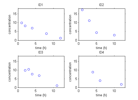
The data can be stored in a table and represented graphically. Here is some simple pharmacokinetics data involving four individuals.
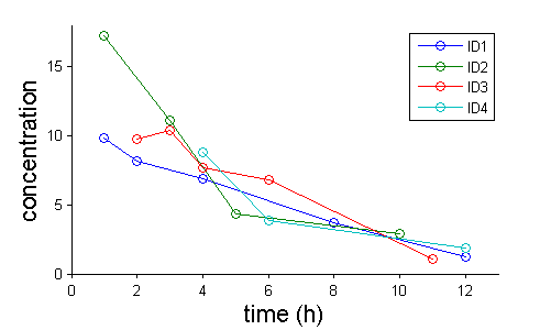
Instead of individual plots, we can plot them all together. Such a figure is usually called a spaghetti plot:
The model
For continuous data, we are going to consider scalar outcomes ($y_{ij}\in \Yr \subset \Rset$) and assume the following general model:
|
(3.1) |
- \( \label{nlme} y_{ij}=f(t_{ij},\bpsi_i)+ g(t_{ij},\bpsi_i)\teps_{ij}, \quad\ 1\leq i \leq N, \ \ 1 \leq j \leq n_i, \)
where $g(t_{ij},\bpsi_i)\geq 0$.
Here, the residual errors $(\teps_{ij})$ are standardized random variables (mean zero and standard deviation 1). In this case, it is clear that $f(t_{ij},\bpsi_i)$ and $g(t_{ij},\bpsi_i)$ are the mean and standard deviation of $y_{ij}$, i.e.,
- \( \begin{array} \esp{y_{ij} | \bpsi_i} &=& f(t_{ij},\bpsi_i) \\ \std{y_{ij} | \bpsi_i} &=& g(t_{ij},\bpsi_i) . \end{array} \)
The structural model
$f$ is known as the {\it structural model} and aims to describe the time evolution of the phenomena under study. For a given subject $i$ and vector of individual parameters $\bpsi_i$, $f(t_{ij},\bpsi_i)$ is the prediction of the observed variable at time $t_{ij}$. In other words, it is the value that would be measured at time $t_{ij}$ if there was no error ($\teps_{ij}=0$).
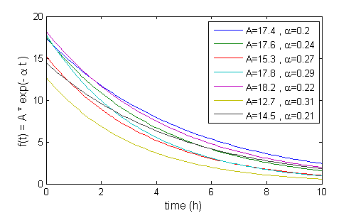
In the current example, we decide to model with the structural model $f=A\exp\left(-\alpha t \right)$. Here are some example curves for various combinations of $A$ and $\alpha$:
Other models involving more complicated dynamical systems can be imagined, such as those defined as solutions of systems of ordinary or partial differential equations. Real-life examples are found in the study of HIV, pharmacokinetics and tumor growth.
The residual error model
For a given structural model $f$, the conditional probability distribution of the observations $(y_{ij})$ is completely defined by the residual error model, i.e., the probability distribution of the residual errors $(\teps_{ij})$ and the standard deviation $g(x_{ij},\bpsi_i)$. The residual error model can take many forms. For example,
- A constant error model assumes that $g(t_{ij},\bpsi_i)=a_i$. Model (3.1) then reduces to
|
(3.2) |
The figure below shows four simulated sequences of observations $(y_{ij}, 1\leq i \leq 4, 1\leq j \leq 10)$ with their respective structural model $f(t,\bpsi_i)$ in blue.
Here, $a_i=2$ is the standard deviation of $y_{ij}$ for all $(i,j)$.
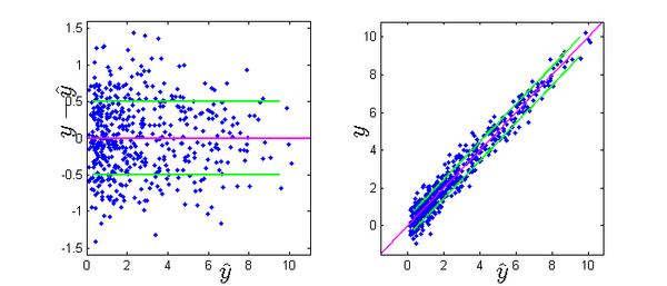
Let $\hat{y}_{ij}=f(t_{ij},\bpsi_i)$ be the prediction of $y_{ij}$ given by the model \eqref{nlme1}. The figure below shows for 50 individuals:
- \emph{left}: prediction errors $e_{ij}=y_{ij}-\hat{y}_{ij}$ vs. predictions $(\hat{y}_{ij})$. The pink line is the mean $\esp{e_{ij}}=0$; the green lines are $\pm$ 1 standard deviations: $\std{e_{ij}}=a_i=2$.
- \emph{right}: observations $(y_{ij})$ vs. predictions $(\hat{y}_{ij})$. The pink line is the identify $y=\hat{y}$, the green lines represent an interval of $\pm 1$ standard deviations around $\hat{y}$: $y=\hat{y}\pm 2$
- These figures are typical for constant error models. The standard deviation of the prediction errors does not depend on the value of the predictions $(\hat{y}_{ij})$, so both intervals have constant amplitude.
- A proportional error model assumes that $g(t_{ij},\bpsi_i) =b_i f(t_{ij},\bpsi_i)$. Model \eqref{nlme} then becomes
|
(3.3) |
The standard deviation of the prediction error $e_{ij}=y_{ij}-\hat{y}_{ij}$ is proportional to the prediction \hbox{$\hat{y}_{ij}$}. Therefore, the amplitude of the $\pm 1$ standard deviation intervals increases linearly with $f$:
[[File:continuous_graf2b.png|600px]]
The standard deviation of the prediction error $e_{ij}$ and thus the amplitude of the intervals are now affine functions of the prediction $\hat{y}_{ij}$:
[[File:continuous_graf2c.png|600px]]
* Another alternative combined error model is $g(t_{ij},\bpsi_i) =\sqrt{a_i^2 + b_i^2 f^2(t_{ij},\bpsi_i)}$.
%
This gives intervals that look fairly similar to the previous ones, though they are no longer affine.
[[File:continuous_graf2d.png|800px]]
<br><br>
=='"`UNIQ--h-5--QINU`"' Extension to autocorrelated errors ==
For any subject $i$, the residual errors $(\teps_{ij},1\leq j \leq n_i)$ are usually assumed to be independent random variables. Extension to autocorrelated errors is possible by assuming for instance that $(\teps_{ij})$ is a stationary ARMA (Autoregressive Moving Average) process.
For example, an autoregressive process of order 1, AR(1), assumes that autocorrelation decreases exponentially:
\begin{equation} \label{autocorr1}
{\rm corr}(\teps_{ij},\teps_{i\,{j+1}}) = \rho_i^{(t_{i\,j+1}-t_{ij})} ,
\end{equation}
where $0\leq \rho_i <1$ for each individual $i$.
If we assume that $t_{ij}=j$ for any $(i,j)$. Then, $t_{i,j+1}-t_{i,j}=1$ and the autocorrelation function $\gamma$ is given by:
\begin{eqnarray*}
\gamma(\tau) &=& {\rm corr}(\teps_{ij},\teps_{i\,j+\tau}) \\ &= &\rho_i^{\tau} .
\end{eqnarray*}
The figure below displays 3 different sequences of residual errors simulated with 3 different autocorrelations $\rho_1=0.1$, $\rho_2=0.6$ and $\rho_3=0.95$. The autocorrelation functions $\gamma(\tau)$ are also displayed.
\includegraphics[width=16cm]{\observationsgraphics/continuous_graf3.png}
\subsubsection{Distribution of the standardized residual errors}
The distribution of the standardized residual errors $(\teps_{ij})$ is usually assumed to be the same for each individual $i$ and any observation time $t_{ij}$.
Furthermore, for identifiability reasons it is also assumed to be symmetrical around 0, i.e., $\prob{\teps_{ij}<-u}=\prob{\teps_{ij}>u}$ for all $u\in \Rset$.
Thus, for any $(i,j)$ the distribution of the observation $y_{ij}$ is also symmetrical around its prediction $f(t_{ij},\bpsi_i)$. This $f(t_{ij},\bpsi_i)$ is therefore both the mean and the median of the distribution of $y_{ij}$: $\esp{y_{ij}|\bpsi_i}=f(t_{ij},\bpsi_i)$ and
$\prob{y_{ij}>f(t_{ij},\bpsi_i)} = \prob{y_{ij}<f(t_{ij},\bpsi_i)} = 1/2$.
If we make the additional hypothesis that 0 is the mode of the distribution of $\teps_{ij}$, then $f(t_{ij},\bpsi_i)$ is also the mode of the distribution of $y_{ij}$.
A widely used bell-shaped distribution for modeling residual errors is the normal distribution. If we assume that $\teps_{ij}\sim {\cal N}(0,1)$, then $y_{ij}$ is also normally distributed: $y_{ij}\sim {\cal N}(f(t_{ij},\bpsi_i),\, g(t_{ij},\bpsi_i))$.
Other distributions can be used, such as \href{http://en.wikipedia.org/wiki/Student's_t-distribution}{Student's $t$-distribution} (also known simply as the $t$-distribution) which is also symmetric and bell-shaped but with heavier tails, meaning that it is more prone to producing values that fall far from its prediction.
\includegraphics[width=10cm]{\observationsgraphics/continuous_graf4.png}
If we assume that $\teps_{ij}\sim t(\nu)$, then
$y_{ij}$ has a non-standardized Student's $t$-distribution.
%%%%%%%%%%%%%%%%%%%%%%%%%%%%%%%%%%%%%
\subsubsection{The conditional likelihood}
The conditional likelihood for given observations $\by$ is defined as
'"`UNIQ-MathJax2-QINU`"'
where $\pcypsi$ is the conditional density function of the observations.
%
If we assume that the residual errors \hbox{$(\teps_{ij},\ 1\leq i \leq N,\ 1\leq j \leq n_i)$} are i.i.d., then the conditional density $\pcypsi$ is straightforward to compute:
\begin{eqnarray}
\label{likeN_model1}
\pcypsi(\by | \bpsi ) & = & \prod_{i=1}^N \pcyipsii(\by_i | \bpsi_i ) \\
& = & \prod_{i=1}^N \prod_{j=1}^{n_i} \pypsiij(y_{ij} | \bpsi_i ) \\
& = & \prod_{i=1}^N \prod_{j=1}^{n_i} \frac{1}{g(t_{ij},\bpsi_i)} \, \peps\left(\frac{y_{ij} - f(t_{ij},\bpsi_i)}{g(t_{ij},\bpsi_i)}\right) ,
\end{eqnarray}
where $\peps$ is the pdf of the i.i.d. residual errors ($\teps_{ij}$).
For example, if we assume that the residual errors $\teps_{ij}$ are Gaussian random variables with mean 0 and variance 1, then
$ \peps(x) = e^{-{x^2}/{2}}/\sqrt{2 \pi}$, and
\begin{eqnarray}
\label{likeN_model2}
\pcypsi(\by | \bpsi ) & = &
\prod_{i=1}^N \prod_{j=1}^{n_i} \frac{1}{\sqrt{2 \pi} g(t_{ij},\bpsi_i)} \, e^{-\frac{1}{2}\left(\frac{y_{ij} - f(t_{ij},\bpsi_i)}{g(t_{ij},\bpsi_i)}\right)^2} .
\end{eqnarray}
\subsubsection{Transforming the data}
The assumption that the distribution of any observation $y_{ij}$ is symmetrical around its predicted value is a very strong one.
If this assumption does not hold, we may decide to transform the data to make it more symmetric around its (transformed) predicted value.
In other cases, constraints on the values that observations can take may also lead us to want to transform the data.
Model \ref{nlme} can be extended to include a transformation of the data:
\begin{eqnarray}\label{def_t}
\transy(y_{ij})=\transy(f(t_{ij},\bpsi_i))+ g(t_{ij},\bpsi_i)\teps_{ij} ,
\end{eqnarray}
where $\transy$ is a monotonic transformation (a strictly increasing or decreasing function).
As you can see, both the data $y_{ij}$ and the structural model $f$ are transformed by the function
$\transy$ so that $f(t_{ij},\bpsi_i)$ remains the prediction of $y_{ij}$.
\vspace{.1cm}
\textbf{Examples:}
\begin{itemize}
\item If $y$ takes non-negative values, a log transformation can be used:
$\transy(y) = \log(y)$.
%Therefore, $y=f e^{g\teps}$.
We can then present the model with one of two equivalent representations:
\begin{eqnarray*}
\log(y_{ij})&=&\log(f(t_{ij},\bpsi_i))+ g(t_{ij},\bpsi_i)\teps_{ij} , \\
y_{ij}&=&f(t_{ij},\bpsi_i)\, e^{ g(t_{ij},\bpsi_i)\teps_{ij} }.
\end{eqnarray*}
\includegraphics[width=16cm]{\observationsgraphics/continuous_graf5a.png}
\item If $y$ takes its values between 0 and 1, a logit transformation can be used:
%\begin{eqnarray*}
%\transy(y)&=&\log(y/(1-y)) \\
% y&=&\frac{f}{f+(1-f) e^{-g\teps}} .
%\end{eqnarray*}
\begin{eqnarray*}
\logit(y_{ij})&=&\logit(f(t_{ij},\bpsi_i))+ g(t_{ij},\bpsi_i)\teps_{ij} , \\
y_{ij}&=& \frac{ f(t_{ij},\bpsi_i) }{ f(t_{ij},\bpsi_i) + (1- f(t_{ij},\bpsi_i)) \, e^{ g(t_{ij},\bpsi_i)\teps_{ij} }}.
\end{eqnarray*}
\includegraphics[width=16cm]{\observationsgraphics/continuous_graf5b.png}
\item The logit error model can be extended if the $y_{ij}$ are known to take their values in an interval $[A,B]$:
\begin{eqnarray*}
\transy(y_{ij})&=&\log((y_{ij}-A)/(B-y_{ij})), \\
y_{ij}&=&A+(B-A)\frac{f(t_{ij},\bpsi_i)-A}{f(t_{ij},\bpsi_i)-A+(B-f(t_{ij},\bpsi_i)) e^{-g(t_{ij},\bpsi_i)\teps_{ij}}}\, .
\end{eqnarray*}
%\includegraphics[width=10cm]{\observationsgraphics/continuous_graf5c.png}
\end{itemize}
Using the transformation proposed in \eq{def_t}, the conditional density $\pcypsi$ becomes
\begin{eqnarray}
\label{likeN_model3}
\pcypsi(\by | \bpsi ) & = & \prod_{i=1}^N \prod_{j=1}^{n_i} \pypsiij(y_{ij} | \bpsi_i ) \\
& = & \prod_{i=1}^N \prod_{j=1}^{n_i} \transy^\prime(y_{ij}) \, \ptypsiij(\transy(y_{ij}) | \bpsi_i ) \\
& = & \prod_{i=1}^N \prod_{j=1}^{n_i} \frac{\transy^\prime(y_{ij})}{g(t_{ij},\bpsi_i)} \, \peps\left(\frac{\transy(y_{ij}) - \transy(f(t_{ij},\bpsi_i))}{g(t_{ij},\bpsi_i)}\right)
\end{eqnarray}
For example, if the observations are log-normally distributed given the individual parameters ($\transy(y) = \log(y)$), with a constant error model ($g(t;\psi_i)=a$), then
'"`UNIQ-MathJax3-QINU`"'
==='"`UNIQ--h-6--QINU`"' Censored data ===
Censoring occurs when the value of a measurement or observation is only partially known.
For continuous data measurements in the longitudinal context, censoring refers to the values of
the measurements, not the times at which they were taken.
For example, in analytical chemistry, the lower limit of detection (LLOD) is the lowest quantity of a substance that can be distinguished from the absence of that substance. Therefore, any time the quantity is below the LLOD, the ``measurement'' is not a number but the information that the quantity is less than the LLOD.
Similarly, in pharmacokinetic studies, measurements of the concentration below a certain limit referred to as the lower limit of quantification (LLOQ) are so low that their reliability is considered suspect.
A measuring device can also have an upper limit of quantification (ULOQ) such that any value above this limit cannot be measured and reported.
As hinted above, censored values are not typically reported as a number, but their existence is known, as well as the type of censoring. Thus, the observation $\repy_{ij}$ (i.e., what is reported) is the measurement $y_{ij}$ if not censored, and the type of censoring otherwise.
We usually distinguish three types of censoring: left, right and interval. We now introduce these, along with illustrative data sets.
\begin{itemize}
\item \emph{Left censoring}: a data point is below a certain value $L$ but it is not known by how much:
'"`UNIQ-MathJax4-QINU`"'
In the figures below, the ``data'' below the limit $L=-0.30$, shown in grey, is not observed. The values are therefore not reported in the dataset.
An additional column \verb!cens! can be used to indicate if an observation is left-censored (\verb!cens=1!) or not (\verb!cens=0!). The column of observations \verb!log-VL! displays the observed log-viral load when it is above the limit $L=-0.30$, and the limit $L=-0.30$ otherwise.
\begin{minipage}{8cm}
\includegraphics[width=8cm]{\observationsgraphics/continuous_graf6a.png}
\end{minipage}
\begin{minipage}{9cm}
{\small
\begin{verbatim}
id time log-VL cens
1 1.0 0.26 0
1 2.0 0.02 0
1 3.0 -0.13 0
1 4.0 -0.13 0
1 5.0 -0.30 1
1 6.0 -0.30 1
1 7.0 -0.25 0
1 8.0 -0.30 1
1 9.0 -0.29 0
1 10.0 -0.30 1
\end{verbatim} }
\end{minipage}
\item \emph{Interval censoring}: if a data point is in interval $I$, its exact value
is not known:
'"`UNIQ-MathJax5-QINU`"'
For example, suppose we are measuring a concentration which naturally only takes non-negative values, but again we cannot measure it below the level $L = 1$. Therefore, any data point $y_{ij}$ below $1$ will be recorded only as ``$y_{ij} \in [0,1)$''.
In the table, an additional column \verb!llimit! is required to indicate the lower bound of the censoring interval.
\begin{minipage}{8cm}
\includegraphics[width=8cm]{\observationsgraphics/continuous_graf6b.png}
\end{minipage}
\begin{minipage}{9cm}
{\small
\begin{verbatim}
id time conc. llimit cens
1 0.3 1.20 . 0
1 0.5 1.93 . 0
1 1.0 3.38 . 0
1 2.0 3.88 . 0
1 4.0 3.24 . 0
1 6.0 1.82 . 0
1 8.0 1.07 . 0
1 12.0 1.00 0.00 1
1 16.0 1.00 0.00 1
1 20.0 1.00 0.00 1
\end{verbatim} }
\end{minipage}
\item \emph{Right censoring}: when a data point is above a certain value $U$, it is not known by how much:
'"`UNIQ-MathJax6-QINU`"'
Column \verb!cens! is used to indicate if an observation is right-censored (\verb!cens=-1!) or not (\verb!cens=0!).
\begin{minipage}{8cm}
\includegraphics[width=8cm]{\observationsgraphics/continuous_graf6c.png}
\end{minipage}
\begin{minipage}{9cm}
{\small
\begin{verbatim}
id time volume cens
1 2.0 1.85 0
1 7.0 2.40 0
1 12.0 3.27 0
1 17.0 3.28 0
1 22.0 3.62 0
1 27.0 3.02 0
1 32.0 3.80 -1
1 37.0 3.80 -1
1 42.0 3.80 -1
1 47.0 3.80 -1
\end{verbatim} }
\end{minipage}
\end{itemize}
{\bf Remarks:}
\begin{itemize}
\item Different censoring limits and intervals can be in play at different times and for different individuals.
\item Interval censoring covers any type of censoring, i.e., setting $I=(-\infty,L]$ for left censoring and $I=[U,+\infty)$ for right censoring.
\end{itemize}
The likelihood needs to be computed carefully in the presence of censored data. To cover all three types of censoring in one go, let $I_{ij}$ be the (finite or infinite) censoring interval existing for individual $i$ at time $t_{ij}$. Then,
\begin{eqnarray}
\label{likeN_model4}
\pcypsi(\brepy | \bpsi ) & = & \prod_{i=1}^N \prod_{j=1}^{n_i} \pypsiij(y_{ij} | \bpsi_i )^{\mathds{1}_{y_{ij} \notin I_{ij}}} \, \prob{y_{ij} \in I_{ij}|\bpsi_i}^{\mathds{1}_{y_{ij} \in I_{ij}}} ,
\end{eqnarray}
where
'"`UNIQ-MathJax7-QINU`"'
We see that if $y_{ij}$ is not censored (i.e., $\mathds{1}_{y_{ij} \notin I_{ij}} = 1$), the contribution to the likelihood is the usual $\pypsiij(y_{ij} | \bpsi_i )$, whereas if it is censored, the contribution is $\prob{y_{ij} \in I_{ij}|\bpsi_i}$.
\subsubsection{Extensions to multidimensional continuous observations}
\begin{itemize}
\item Extension to multidimensional observations is straightforward. If $d$ outcomes are simultaneously measured at $t_{ij}$, then $y_{ij}$ is a now a vector in $\Rset^d$ and we can suppose that equation \eqref{nlme} still holds for each component of $y_{ij}$. Thus, for $1\leq m \leq d$,
\begin{equation}
y_{ijm}=f_m(t_{ij},\bpsi_i)+ g_m(t_{ij},\bpsi_i)\teps_{ijm} , \ \ 1\leq i \leq N,
\ \ 1 \leq j \leq n_i.
\end{equation}
It is then possible to introduce correlation between the components of each observation by assuming that \hbox{$\teps_{ij} = (\teps_{ijm} , 1\leq m \leq d)$} is a random vector with mean 0 and correlation matrix $R_{\teps_{ij}}$.
\item Suppose instead that $K$ replicates of the same measurement are taken at time $t_{ij}$. Then, the model becomes, for $1 \leq k \leq K$,
\begin{equation}
y_{ijk}=f(t_{ij},\bpsi_i)+ g(t_{ij},\bpsi_i)\teps_{ijk} ,\ \ 1\leq i \leq N,
\ \ 1 \leq j \leq n_i .
\end{equation}
Following what can be done for decomposing random effects into inter-individual and inter-occasion components, we can decompose the residual error into inter-measurement and inter-replicate components:
\begin{equation}
y_{ijk}=f(t_{ij},\bpsi_i)+ g_{I\!M}(t_{ij},\bpsi_i)\vari{\teps}{ij}{I\!M} + g_{I\!R}(x_{ij},\bpsi_i)\vari{\teps}{ijk}{I\!R} .
\end{equation}
\end{itemize}
\subsubsection{Summary}
\setlength{\fboxsep}{5mm}
%\setlength{\fboxrule}{1mm}
\fbox{\begin{minipage}{0.7\textwidth}
A model for continuous data is completely defined by:
\begin{itemize}
\item the structural model $f$
\item the residual error model $g$
\item the probability distribution of the residual errors $(\teps_{ij})$
\item \possibly a transformation $\transy$ of the data
\end{itemize}
\vspace{.2cm}
The model is associated with a design which includes:
\begin{itemize}
\item the observation times $(t_{ij})$
\item \possibly some additional regression variables $(x_{ij})$
\item \possibly the inputs $(u_i)$ (e.g., the dosing regimen for a PK model)
\item \possibly a censoring process $(I_{ij})$
\end{itemize}
\end{minipage}}
\vspace*{1cm}
\hrule
\subsubsection{MLXtran for continuous data models}
{\bf Example 1:}
\begin{minipage}{0.45\textwidth}
\begin{eqnarray*}
\psi &=& (A,\alpha,B,\beta, a) \\
f(t,\psi) &=& A\, e^{- \alpha \, t} + B\, e^{- \beta \, t} \\
y_{ij} &=& f(t_{ij} , \psi_i) + a\, \teps_{ij}
\end{eqnarray*}
\end{minipage}
\begin{minipage}{0.55\textwidth}
%\begin{Verbatim}[frame=single,fontsize=\small]
\begin{lstlisting}[frame=trBL,linewidth=10cm]
INPUT:
input = {A, B, alpha, beta, a}
EQUATION:
f = A*exp(-alpha*t) + B*exp(-beta*t)
DEFINITION:
y = {distribution=normal, prediction=f, std=a}
\end{lstlisting}
%\end{Verbatim}
\end{minipage}
\medskip
{\bf Example 2:}
\begin{minipage}{0.45\textwidth}
\begin{eqnarray*}
\psi &=& (\delta, c , \beta, p, s, d, \nu,\rho, a) \\
t_0 &=&0 \\[0.4cm]
\mbox{if $t<t_0$} \\
\nitc &=& \delta \, c/( \beta \, p) \\
\itc &=& (s - d\,\nitc) / \delta \\
\vl &=& p \, \itc / c. \\ \mbox{else } \quad\\
 \dA{\nitc}{} & = & s - \beta(1-\nu) \, \nitc(t) \, \vl(t) - d\,\nitc(t)  \\
 \dA{\itc}{} & = & \beta(1-\nu) \, \nitc(t) \, \vl(t) - \delta \, \itc(t) \\
 \dA{\vl}{} & = & p(1-\rho) \, \itc(t) - c \, \vl(t) \\[0.3cm]
\log(y_{ij}) &= &\log(V(t_{ij} , \psi_i)) + a\, \teps_{ij} \end{eqnarray*} \end{minipage} \begin{minipage}{0.55\textwidth} %\begin{Verbatim}[frame=single,fontsize=\small,xleftmargin=0mm] \begin{lstlisting}[frame=trBL,linewidth=10cm] INPUT: input = {delta, c, beta, p, s, d, nu, rho, a} EQUATION: t0=0 N_0 = delta*c/(beta*p) I_0 = (s - d*N_0)/delta V_0 = p*I_0/c ddt_N = s - beta*(1-nu)*N*V - d*N ddt_I = beta*(1-nu)*N*V - delta*I ddt_V = p*(1-rho)*I - c*V DEFINITION: y = {distribution=logNormal, prediction=V, std=a} \end{lstlisting} %\end{Verbatim} \end{minipage}
%\cleardoublepage
%\phantomsection
%\addcontentsline{toc}{subsection}{Bibliography}
\vskip 1cm
\bibliographystyle{plainnat} \bibliography{../../bibtex/general} %\bibliography{bibliodir} %\bibliography{D:/Book/biblio/bibtex}


