Difference between revisions of "The individual approach"
m |
m |
||
| Line 31: | Line 31: | ||
| − | Maximum likelihood estimation of the parameters: $\hat{\psi}$ maximizes $L(\psi ; y_1,y_2,\ldots,y_j) | + | Maximum likelihood estimation of the parameters: $\hat{\psi}$ maximizes $L(\psi ; y_1,y_2,\ldots,y_j)$ |
where | where | ||
Revision as of 12:46, 29 January 2013
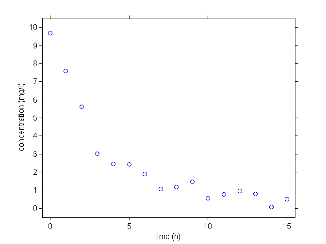
An example of continuous data from a single individual
A model for continuous data:
\begin{eqnarray*}
y_{j} &=& f(t_j ; \psi) + \varepsilon_j \quad ; \quad 1\leq j \leq n \\ \\
&=& f(t_j ; \psi) + g(t_j ; \psi) \bar{\varepsilon_j}
\end{eqnarray*}
- $f$ : structural model
- $\psi=(\psi_1, \psi_2, \ldots, \psi_d)$ : vector of parameters
- $(t_1,t_2,\ldots , t_n)$ : observation times
- $(\varepsilon_j, \varepsilon_2, \ldots, \varepsilon_n)$ : residual errors ($\Epsilon({\varepsilon_j}) =0$)
- $g$ : { residual error model}
- $(\bar{\varepsilon_1}, \bar{\varepsilon_2}, \ldots, \bar{\varepsilon_n})$ : normalized residual errors (Var({\bar{\varepsilon_j}}) =1)
Some tasks in the context of modelling, {\i.e.} when a vector of observations $(y_j)$ is available:
- Simulate a vector of observations $(y_j)$ for a given model and a given parameter $\psi$,
- Estimate the vector of parameters $\psi$ for a given model,
- Select the structural model $f$
- Select the residual error model $g$
- Assess/validate the selected model
Maximum likelihood estimation of the parameters: $\hat{\psi}$ maximizes $L(\psi ; y_1,y_2,\ldots,y_j)$
where \begin{equation} L(\psi ; y_1,y_2,\ldots,y_j) {\overset{def}{=}} p_Y( y_1,y_2,\ldots,y_j ; \psi) \end{equation}
If we assume that $\bar{\varepsilon_i} \sim_{i.i.d} {\cal N}(0,1)$, then, the $y_i$'s are independent and
\begin{equation} y_{j} \sim {\cal N}(f(t_j ; \psi) , g(t_j ; \psi)^2) \end{equation}
and the p.d.f of $(y_1, y_2, \ldots y_n)$ can be computed:
\begin{eqnarray*}
p_Y(y_1, y_2, \ldots y_n ; \psi) &=& \prod_{j=1}^n p_{Y_j}(y_j ; \psi) \\ \\
&& \frac{e^{-\frac{1}{2} \sum_{j=1}^n \left( \frac{y_j - f(t_j ; \psi)}{g(t_j ; \psi)} \right)^2}}{\prod_{j=1}^n \sqrt{2\pi g(t_j ; \psi)}}
\end{eqnarray*}
Maximizing the likelihood is equivalent to minimizing the deviance (-2 $\times$ log-likelihood) which plays here the role of the objective function: \begin{equation} \hat{\psi} = \DeclareMathOperator*{\argmin}{arg\,min}_{\psi} \left\{ \sum_{j=1}^n \log(g(t_j ; \psi)^2) + \sum_{j=1}^n \left( \frac{y_j - f(t_j ; \psi)}{g(t_j ; \psi) }\right)^2 \right \} \end{equation}
and the deviance is therefore
\begin{eqnarray*}
-2 LL(\hat{\psi} ; y_1,y_2,\ldots,y_j) = \sum_{j=1}^n \log(g(t_j ; \hat{\psi})^2) + \sum_{j=1}^n \left(\frac{y_j - f(t_j ; \hat{\psi})}{g(t_j ; \hat{\psi})}\right)^2 +n\log(2\pi)
\end{eqnarray*}
This minimization problem usually does not have an analytical solution for a non linear model. Some optimization procedure should be used.
For a constant error model ($y_{j} = f(t_j ; \phi) + a \, \teps_j$), we have \begin{eqnarray*} \hat{\phi} &=& \argmin{\psi} \sum_{j=1}^n \left( y_j - f(t_j ; \phi)\right)^2 \\ \hat{a}&=& \frac{1}{n}\sum_{j=1}^n \left( y_j - f(t_j ; \hat{\phi})\right)^2 \\ -2 LL(\hat{\psi} ; y_1,y_2,\ldots,y_j) &=& \sum_{j=1}^n \log(\hat{a}^2) + n +n\log(2\pi) \end{eqnarray*}
A linear model has the form \begin{equation} y_{j} = F \, \phi + a \, \teps_j \end{equation}
The solution has then a close form \begin{eqnarray*} \hat{\phi} &=& (F^\prime F)^{-1} F^\prime y \\ \hat{a}&=& \frac{1}{n}\sum_{j=1}^n \left( y_j - F \hat{\phi})\right)^2 \end{eqnarray*}
A PK example
A dose of 100 mg of a drug is administrated to a patient as an intravenous (IV) bolus at time 0 and concentrations of the drug are measured every hour during 15 hours.
We consider the three following structural models:
- One compartment model
\begin{equation} f_1(t ; V,k_e) = \frac{D}{V} e^{-k_e \, t} '"`UNIQ-MathJax1-QINU`"' \end{equation}
- Polynomial model
$$ f_3(t ; V,\alpha,\beta,\gamma) = \frac{1}{V}(D-\alpha t - \beta t^2 - \gamma t^3) $$
and the four following residual error models:
