The individual approach

Overview

Before we start looking at modeling a whole population at the same time, we are going to consider only one individual from that population. Much of the basic methodology for modeling one individual follows through to population modeling. We will see that when stepping up from one individual to a population, the difference is that some parameters shared by individuals are considered to be drawn from a probability distribution.

Let us begin with a simple example. An individual receives 100mg of a drug at time $t=0$. At that time and then every hour for fifteen hours, the concentration of a marker in the bloodstream is measured and plotted against time:

We aim to find a mathematical model to describe what we see in the figure. The eventual goal is then to extend this approach to the simultaneous modeling of a whole population.

Model and methods for the individual approach

Defining a model

In our example, the concentration is a continuous variable, so we will try to use continuous functions to model it. Different types of data (e.g., count data, categorical data, time-to-event data, etc.) require different types of models. All of these data types will be considered in due time, but for now let us concentrate on a continuous data model.

A model for continuous data can be represented mathematically as follows:

where:

• $f$ is called the structural model. It corresponds to the basic type of curve we suspect the data is following, e.g., linear, logarithmic, exponential, etc. Sometimes, a model of the associated biological processes leads to equations that define the curve's shape.

• $(t_1,t_2,\ldots , t_n)$ is the vector of observation times. Here, $t_1 = 0$ hours and $t_n = t_{16} = 15$ hours.

• $\psi=(\psi_1, \psi_2, \ldots, \psi_d)$ is a vector of $d$ parameters that influences the value of $f$.

• $(e_1, e_2, \ldots, e_n)$ are called the residual errors. Usually, we suppose that they come from some centered probability distribution: $\esp{e_j} =0$.

In fact, we usually state a continuous data model in a slightly more flexible way:

\( y_{j} = f(t_j ; \psi) + g(t_j ; \psi)\teps_j , \quad \quad 1\leq j \leq n, \)

(1)

where now:

• $g$ is called the residual error model. It may be a function of the time $t_j$ and parameters $\psi$.
• $(\teps_1, \teps_2, \ldots, \teps_n)$ are the normalized residual errors. We suppose that these come from a probability distribution which is centered and has unit variance: $\esp{\teps_j} = 0$ and $\var{\teps_j} =1$.

Choosing a residual error model

The choice of a residual error model $g$ is very flexible, and allows us to account for many different hypotheses we may have on the error's distribution. Let $f_j=f(t_j;\psi)$. Here are some simple error models.

• Constant error model: $g=a$. That is, $y_j=f_j+a\teps_j$.
• Proportional error model: $g=b\,f$. That is, $y_j=f_j+bf_j\teps_j$. This is for when we think the magnitude of the error is proportional to the value of the predicted value $f$.
• Combined error model: $g=a+b f$. Here, $y_j=f_j+(a+bf_j)\teps_j$.
• Alternative combined error model: $g^2=a^2+b^2f^2$. Here, $y_j=f_j+\sqrt{a^2+b^2f_j^2}\teps_j$.
• Exponential error model: here, the model is instead $\log(y_j)=\log(f_j) + a\teps_j$, that is, $g=a$. It is exponential in the sense that if we exponentiate, we end up with $y_j = f_j e^{a\teps_j}$.

Tasks

To model a vector of observations $y = (y_j,\, 1\leq j \leq n$) we must perform several tasks:

• Select a structural model $f$ and a residual error model $g$.
• Estimate the model's parameters $\psi$.
• Assess and validate the selected model.

Selecting structural and residual error models

As we are interested in parametric modeling, we must choose parametric structural and residual error models. In the absence of biological (or other) information, we might suggest possible structural models just by looking at the graphs of time-evolution of the data. For example, if $y_j$ is increasing with time, we might suggest an affine, quadratic or logarithmic model, depending on the approximate trend of the data. If $y_j$ is instead decreasing ever slower to zero, an exponential model might be appropriate.

However, often we have biological (or other) information to help us make our choice. For instance, if we have a system of differential equations describing how the drug is eliminated from the body, its solution may provide the formula (i.e., structural model) we are looking for.

As for the residual error model, if it is not immediately obvious which one to choose, several can be tested in conjunction with one or several possible structural models. After parameter estimation, each structural and residual error model pair can be assessed, compared against the others, and/or validated in various ways.

Now we can have a first look at parameter estimation, and further on, model assessment and validation.

Parameter estimation

Given the observed data and the choice of a parametric model to describe it, our goal becomes to find the "best" parameters for the model. A traditional framework to solve this kind of problem is called maximum likelihood estimation or MLE, in which the "most likely" parameters are found, given the data that was observed.

The likelihood $L$ is a function defined as:

i.e., the conditional joint density function of $(y_j)$ given the parameters $\psi$, but looked at as if the data are known and the parameters not. The $\hat{\psi}$ which maximizes $L$ is known as the maximum likelihood estimator.

Suppose that we have chosen a structural model $f$ and residual error model $g$. If we assume for instance that $ \teps_j \sim_{i.i.d} {\cal N}(0,1)$, then the $y_j$ are independent of each other and (1) means that:

Due to this independence, the pdf of $y = (y_1, y_2, \ldots, y_n)$ is the product of the pdfs of each $y_j$:

This is the same thing as the likelihood function $L$ when seen as a function of $\psi$. Maximizing $L$ is equivalent to minimizing the deviance, i.e., -2 $\times$ the $\log$-likelihood ($LL$):

\(\begin{eqnarray} \hat{\psi} &=& \argmin{\psi} \left\{ -2 \,LL \right\}\\ &=& \argmin{\psi} \left\{ \sum_{j=1}^n \log\left(g(t_j ; \psi)^2\right) + \sum_{j=1}^n \left(\displaystyle{ \frac{y_j - f(t_j ; \psi)}{g(t_j ; \psi)} }\right)^2 \right\} . \end{eqnarray}\)

(2)

This minimization problem does not usually have an analytical solution for nonlinear models, so an optimization procedure needs to be used. However, for a few specific models, analytical solutions do exist.

For instance, suppose we have a constant error model: $y_{j} = f(t_j ; \psi) + a \, \teps_j,\,\, 1\leq j \leq n,$ that is: $g(t_j;\psi) = a$. In practice, $f$ is not itself a function of $a$, so we can write $\psi = (\phi,a)$ and therefore: $y_{j} = f(t_j ; \phi) + a \, \teps_j.$ Thus, (2) simplifies to:

The solution is then:

where $\hat{a}^2$ is found by setting the partial derivative of $-2LL$ to zero.

Whether this has an analytical solution or not depends on the form of $f$. For example, if $f(t_j;\phi)$ is just a linear function of the components of the vector $\phi$, we can represent it as a matrix $F$ whose $j$th row gives the coefficients at time $t_j$. Therefore, we have the matrix equation $y = F \phi + a \teps$.

The solution for $\hat{\phi}$ is thus the least-squares one, and for $\hat{a}^2$ it is the same as before:

Computing the Fisher information matrix

The Fisher information is a way of measuring the amount of information that an observable random variable carries about an unknown parameter upon which its probability distribution depends.

Let $\psis $ be the true unknown value of $\psi$, and let $\hatpsi$ be the maximum likelihood estimate of $\psi$. If the observed likelihood function is sufficiently smooth, asymptotic theory for maximum-likelihood estimation holds and

\( I_n(\psis)^{\frac{1}{2} }(\hatpsi-\psis) \limite{n\to \infty}{} {\mathcal N}(0,\id) , \)

(3)

where $I_n(\psis)$ is (minus) the Hessian (i.e., the matrix of the second derivatives) of the log-likelihood:

is the observed Fisher information matrix. Here, "observed" means that it is a function of observed variables $y_1,y_2,\ldots,y_n$.

Thus, an estimate of the covariance of $\hatpsi$ is the inverse of the observed Fisher information matrix as expressed by the formula:

Deriving confidence intervals for parameters

Let $\psi_k$ be the $k$th of $d$ components of $\psi$. Imagine that we have estimated $\psi_k$ with $\hatpsi_k$, the $k$th component of the MLE $\hatpsi$, that is, a random variable that converges to $\psi_k^{\star}$ when $n \to \infty$ under very general conditions.

An estimator of its variance is the $k$th element of the diagonal of the covariance matrix $C(\hatpsi)$:

We can thus derive an estimator of its standard error:

and a confidence interval of level $1-\alpha$ for $\psi_k^\star$:

where $q(w)$ is the quantile of order $w$ of a ${\cal N}(0,1)$ distribution.

Deriving confidence intervals for predictions

The structural model $f$ can be predicted for any $t$ using the estimated value $f(t; \hatphi)$. For that $t$, we can then derive a confidence interval for $f(t,\phi)$ using the estimated variance of $\hatphi$. Indeed, as a first approximation we have:

where $\nabla f(t,\phis)$ is the gradient of $f$ at $\phis$, i.e., the vector of the first-order partial derivatives of $f$ with respect to the components of $\phi$, evaluated at $\phis$. Of course, we do not actually know $\phis$, but we can estimate $\nabla f(t,\phis)$ with $\nabla f(t,\hatphi)$. The variance of $f(t ; \hatphi)$ can then be estimated by

We can then derive an estimate of the standard error of $f (t,\hatphi)$ for any $t$:

and a confidence interval of level $1-\alpha$ for $f(t ; \phi^\star)$:

Estimating confidence intervals using Monte Carlo simulation

The use of Monte Carlo methods to estimate a distribution does not require any approximation of the model.

We proceed in the following way. Suppose we have found a MLE $\hatpsi$ of $\psi$. We then simulate a data vector $y^{(1)}$ by first randomly generating the vector $\teps^{(1)}$ and then calculating for $1 \leq j \leq n$,

In a sense, this gives us an example of "new" data from the "same" model. We can then compute a new MLE $\hat{\psi}^{(1)}$ of $\psi$ using $y^{(1)}$.

Repeating this process $M$ times gives $M$ estimates of $\psi$ from which we can obtain an empirical estimation of the distribution of $\hatpsi$, or any quantile we like.

Any confidence interval for $\psi_k$ (resp. $f(t,\psi_k)$) can then be approximated by a prediction interval for $\hatpsi_k$ (resp. $f(t,\hatpsi_k)$). For instance, a two-sided confidence interval of level $1-\alpha$ for $\psi_k^\star$ can be estimated by the prediction interval

where $[\cdot]$ denotes the integer part and $(\psi_{k,(m)},\ 1 \leq m \leq M)$ the order statistic, i.e., the parameters $(\hatpsi_k^{(m)}, 1 \leq m \leq M)$ reordered so that $\hatpsi_{k,(1)} \leq \hatpsi_{k,(2)} \leq \ldots \leq \hatpsi_{k,(M)}$.

A PK example

In the real world, it is often not enough to look at the data, choose one possible model and estimate the parameters. The chosen structural model may or may not be "good" at representing the data. It may be good but the chosen residual error model bad, meaning that the overall model is poor, and so on. That is why in practice we may want to try out several structural and residual error models. After performing parameter estimation for each model, various assessment tasks can then be performed in order to conclude which model is best.

The data

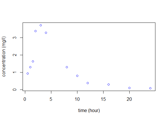
This modeling process is illustrated in detail in the following PK example. Let us consider a dose D=50mg of a drug administered orally to a patient at time $t=0$. The concentration of the drug in the bloodstream is then measured at times $(t_j) = (0.5, 1,\,1.5,\,2,\,3,\,4,\,8,\,10,\,12,\,16,\,20,\,24).$ Here is the file individualFitting_data.txt with the data:

Time	Concentration
0.5	0.94
1.0	1.30
1.5	1.64
2.0	3.38
3.0	3.72
4.0	3.29
8.0	1.31
10.0	0.80
12.0	0.39
16.0	0.31
20.0	0.10
24.0	0.09

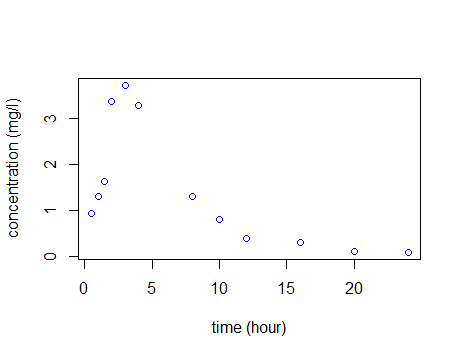
We are going to perform the analyses for this example with the free statistical software R. First, we import the data and plot it to have a look:

Fitting two PK models

We are going to consider two possible structural models that may describe the observed time-course of the concentration:

• A one compartment model with first-order absorption and linear elimination:




• A one compartment model with zero-order absorption and linear elimination:

We define each of these functions in R:

We then define two models ${\cal M}_1$ and ${\cal M}_2$ that assume (for now) constant residual error models:

We can fit these two models to our data by computing the MLE $\hatpsi_1=(\hatphi_1,\hat{a}_1)$ and $\hatpsi_2=(\hatphi_2,\hat{a}_2)$ of $\psi$ under each model:

Here are the parameter estimation results:

Assessing and selecting the PK model

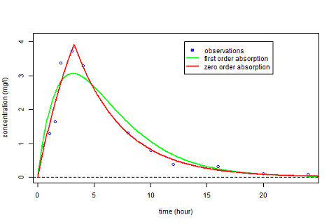
The estimated parameters $\hatphi_1$ and $\hatphi_2$ can then be used for computing the predicted concentrations $\hat{f}_1(t)$ and $\hat{f}_2(t)$ under both models at any time $t$. These curves can then be plotted over the original data and compared:

We clearly see that a much better fit is obtained with model ${\cal M}_2$, i.e., the one assuming a zero-order absorption process.

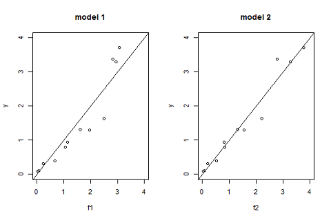
Another useful goodness-of-fit plot is obtained by displaying the observations $(y_j)$ versus the predictions $\hat{y}_j=f(t_j ; \hatpsi)$ given by the models:

Model selection

Again, ${\cal M}_2$ would seem to have a slight edge. This can be tested more analytically using the Bayesian Information Criteria (BIC):

A smaller BIC is better. Therefore, this also suggests that model ${\cal M}_2$ should be selected.

Fitting different error models

For the moment, we have only considered constant error models. However, the "observations vs predictions" figure hints that the amplitude of the residual errors may increase with the size of the predicted value. Let us therefore take a closer look at four different residual error models, each of which we will associate with the "best" structural model $f_2$:

${\cal M}_2$	Constant error model:	$y_j=f_2(t_j;\phi_2)+a_2\teps_j$
${\cal M}_3$	Proportional error model:	$y_j=f_2(t_j;\phi_3)+b_3f_2(t_j;\phi_3)\teps_j$
${\cal M}_4$	Combined error model:	$y_j=f_2(t_j;\phi_4)+(a_4+b_4f_2(t_j;\phi_4))\teps_j$
${\cal M}_5$	Exponential error model:	$\log(y_j)=\log(f_2(t_j;\phi_5)) + a_5\teps_j$.

The three new ones need to be entered into R:

We can now compute the MLE $\hatpsi_3=(\hatphi_3,\hat{b}_3)$, $\hatpsi_4=(\hatphi_4,\hat{a}_4,\hat{b}_4)$ and $\hatpsi_5=(\hatphi_5,\hat{a}_5)$ of $\psi$ under models ${\cal M}_3$, ${\cal M}_4$ and ${\cal M}_5$:

Selecting the error model

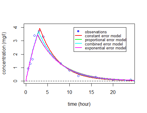
As before, these curves can be plotted over the original data and compared:

As you can see, the three predicted concentrations obtained with models ${\cal M}_3$, ${\cal M}_4$ and ${\cal M}_5$ are quite similar. We now calculate the BIC for each:

All of these BIC are lower than the constant residual error one. BIC selects the residual error model ${\cal M}_3$ with a proportional component.

There is not a large difference between these three error models, though the proportional and combined error models give the smallest and essentially identical BIC. We decide to use the combined error model ${\cal M}_4$ in the following (the same types of analysis could be done with the proportional error model).

A 90% confidence interval for $\psi_4$ can derived from the Hessian (i.e., the square matrix of second-order partial derivatives) of the objective function (i.e. -2 $\times \ LL$):

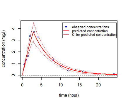
We can also calculate a 90% confidence interval for $f_4(t)$ using the Central Limit Theorem (see (3)):

This can then be plotted:

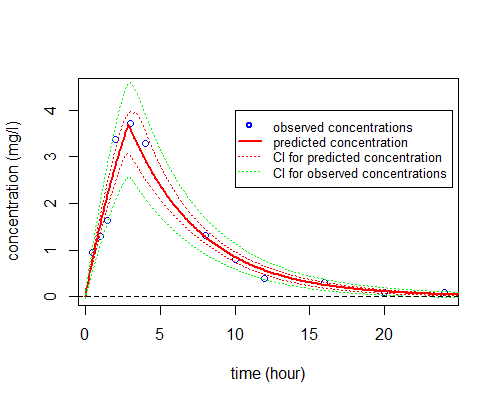
Alternatively, prediction intervals for $\hatpsi_4$, $\hat{f}_4(t;\hatpsi_4)$ and new observations for any time $t$ can be estimated by Monte Carlo simulation:

The R code and input data used in this section can be downloaded here: https://wiki.inria.fr/wikis/popix/images/a/a1/R_IndividualFitting.rar.

Bibliography

Buonaccorsi, J.P. - Measurement Error: Models, Methods, and Applications

Taylor & Francis,2010

http://books.google.fr/books?id=QVtVmaCqLHMC
Bibtex

Author : Buonaccorsi, J.P.
Title : Measurement Error: Models, Methods, and Applications
In : -
Address :
Date : 2010

Carroll, R.J., Ruppert, D., Stefanski, L.A., Crainiceanu, C.M. - Measurement Error in Nonlinear Models: A Modern Perspective, Second Edition

Taylor & Francis,2010

http://books.google.fr/books?id=9kBx5CPZCqkC
Bibtex

Author : Carroll, R.J., Ruppert, D., Stefanski, L.A., Crainiceanu, C.M.
Title : Measurement Error in Nonlinear Models: A Modern Perspective, Second Edition
In : -
Address :
Date : 2010

Fitzmaurice, G.M., Laird, N.M., Ware, J.H. - Applied Longitudinal Analysis

Wiley,2004

http://books.google.fr/books?id=gCoTIFejMgYC
Bibtex

Author : Fitzmaurice, G.M., Laird, N.M., Ware, J.H.
Title : Applied Longitudinal Analysis
In : -
Address :
Date : 2004

Gallant, A.R. - Nonlinear Statistical Models

Wiley,2009

http://books.google.fr/books?id=imv-NMozseEC
Bibtex

Author : Gallant, A.R.
Title : Nonlinear Statistical Models
In : -
Address :
Date : 2009

Huet, S., Bouvier, A., Poursat, M.A., Jolivet, E. - Statistical tools for nonlinear regression: a practical guide with S-PLUS and R examples

Springer,2003

Bibtex

Author : Huet, S., Bouvier, A., Poursat, M.A., Jolivet, E.
Title : Statistical tools for nonlinear regression: a practical guide with S-PLUS and R examples
In : -
Address :
Date : 2003

Ritz, C., Streibig, J.C. - Nonlinear regression with R

Vol. 33, Springer New York,2008

Bibtex

Author : Ritz, C., Streibig, J.C.
Title : Nonlinear regression with R
In : -
Address :
Date : 2008

Ross, G.J.S. - Nonlinear estimation

Springer-Verlag,1990

http://books.google.fr/books?id=7LkyzdLMghIC
Bibtex

Author : Ross, G.J.S.
Title : Nonlinear estimation
In : -
Address :
Date : 1990

Seber, G.A.F., Wild, C.J. - Nonlinear Regression

Wiley,2003

http://books.google.fr/books?id=YBYlCpBNo\_cC
Bibtex

Author : Seber, G.A.F., Wild, C.J.
Title : Nonlinear Regression
In : -
Address :
Date : 2003

Serroyen, J., Molenberghs, G., Verbeke, G., Davidian, M. - Nonlinear models for longitudinal data

The American Statistician 63(4):378-388,2009

Bibtex

Author : Serroyen, J., Molenberghs, G., Verbeke, G., Davidian, M.
Title : Nonlinear models for longitudinal data
In : The American Statistician -
Address :
Date : 2009

Wolberg, J.R. - Data analysis using the method of least squares: extracting the most information from experiments

Vol. 1, Springer Berlin, Germany,2006

Bibtex

Author : Wolberg, J.R.
Title : Data analysis using the method of least squares: extracting the most information from experiments
In : -
Address :
Date : 2006

Overview	What is a model? A joint probability distribution!