Difference between revisions of "Estimation of the log-likelihood"
m (→Estimation using importance sampling) |
m |
||
| Line 26: | Line 26: | ||
Thus, $\pyi(y_i;\theta)$ is expressed as a mean. It can therefore be approximated by an empirical mean using a Monte Carlo procedure: | Thus, $\pyi(y_i;\theta)$ is expressed as a mean. It can therefore be approximated by an empirical mean using a Monte Carlo procedure: | ||
| + | |||
<blockquote> | <blockquote> | ||
| Line 68: | Line 69: | ||
We can now approximate $\pyi(y_i;\theta)$ via an ''importance sampling'' integration method using $\tqphii$ as a proposal distribution: | We can now approximate $\pyi(y_i;\theta)$ via an ''importance sampling'' integration method using $\tqphii$ as a proposal distribution: | ||
| + | |||
<blockquote> | <blockquote> | ||
Revision as of 14:35, 21 May 2013
Estimation using importance sampling
The observed log-likelihood ${\llike}(\theta;\by)=\log({\like}(\theta;\by))$ can be estimated without requiring approximation of the model, using a Monte-Carlo approach.
Since
we can estimate $\log(\pyi(y_i;\theta))$ for each individual and derive an estimate of the log-likelihood as the sum of these individual log-likelihoods. We will now explain how to estimate $\log(\pyi(y_i;\theta))$ for any individual $i$.
Using the $\phi$-representation of the model, notice first that $\pyi(y_i;\theta)$ can be decomposed as follows:
Thus, $\pyi(y_i;\theta)$ is expressed as a mean. It can therefore be approximated by an empirical mean using a Monte Carlo procedure:
1. Draw $M$ independent values $\phi_i^{(1)}$, $\phi_i^{(2)}$, ..., $\phi_i^{(M)}$ from the normal distribution $\qphii(\, \cdot \, ; \theta)$.
2. Estimate $ \pyi(y_i;\theta)$ with
By construction, this estimator is unbiased:
Furthermore, it is consistent since its variance decreases as $1/M$:
We could consider ourselves satisfied with this estimator since we "only" have to select $M$ large enough to get an estimator with a small variance. Nevertheless, we will see now that it is possible to improve the statistical properties of this estimator.
For any distribution $\tqphii$ that is absolutely continuous with respect to the marginal distribution $\qphii$, we can write
We can now approximate $\pyi(y_i;\theta)$ via an importance sampling integration method using $\tqphii$ as a proposal distribution:
1. Draw $M$ independent values $\phi_i^{(1)}$, $\phi_i^{(2)}$, ..., $\phi_i^{(M)}$ from the proposal distribution $\tqphii(\, \cdot \, ; \theta)$.
2. Estimate $ \pyi(y_i;\theta)$ with
By construction, this new estimator is also unbiased and its variance also decreases as $1/M$:
There exists an infinite number of possible proposal distributions $\tpphii$ which all provide the same rate of convergence $1/M$. The trick is to reduce the variance of the estimator by selecting a proposal distribution so that the numerator is as small as possible.
Imagine that we use the conditional distribution $\qcphiiyi$ as the proposal. Then, for any $m=1,2,\ldots,M$,
which means that $\hat{p}_{i,M}=\pyi(y_i;\theta)$! Such an estimator is optimal since its variance is null and only one realization of $\qcphiiyi$ is required to exactly compute $\pyi(y_i;\theta)$. The problem is that it is not possible to generate the $\phi_i^{(m)}$ with this conditional distribution, since that would require to compute a normalizing constant, which here is precisely $\pyi(y_i;\theta)$.
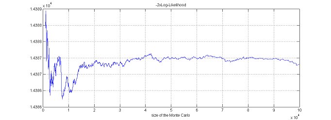
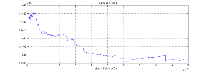
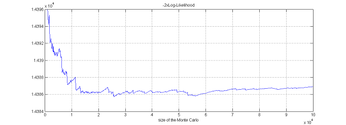
Nevertheless, this conditional distribution can be estimated using the Metropolis-Hastings algorithm described in The Metropolis-Hastings algorithm for simulating the individual parameters Section and a practical proposal "close" to the optimal proposal $\qcphiiyi$ can be derived. We can then expect to get a very accurate estimate with a relatively small Monte Carlo size $M$.
In $\monolix$, the mean and variance of the conditional distribution $\qcphiiyi$ are estimated by Metropolis-Hastings for each individual $i$. Then, the $\phi_i^{(m)}$ are drawn with a noncentral $t$ distribution:
where $\mu_i$ and $\sigma^2_i$ are estimates of $\esp{\phi_i|y_i;\theta}$ and $\var{\phi_i|y_i;\theta}$, and $(T_{i,m})$ is a sequence of i.i.d. random variables distributed with a Student's $t$ distribution with $\nu$ degrees of freedom.
$\monolix$ uses the default value $\nu=5$. It is also possible to automatically test different degrees of freedom from the set $\{2, 5, 10, 20\}$ and to select the one that provides the smallest empirical variance for $\widehat{ {\llike} }_M(\theta;\by) = \sum_{i=1}^{N}\log(\hat{p}_{i,M})$.
Estimation using linearization
For continuous data models, an alternative to the importance sampling approach is to use a linearization of the model like that proposed in the Estimation of the F.I.M. using a linearization of the model Section to approximate the observed Fisher Information Matrix. Indeed, the marginal distribution of a continuous vector of observations $y_i$ can be approximated by a normal distribution. It is then straightforward to derive the associated likelihood. All of these calculations are described in the Estimation of the F.I.M. using a linearization of the model Section.
This method can be much faster than importance sampling. It should be used by modelers for model selection purposes during the initial runs, when the goal is to identify significant differences between models. Importance sampling should be used when a more precise evaluation of the log-likelihood is required.


