Difference between revisions of "The SAEM algorithm for estimating population parameters"
m |
m |
||
| Line 6: | Line 6: | ||
The SAEM (Stochastic Approximation of EM) algorithm is a stochastic algorithm for calculating the maximum likelihood estimator (MLE) in the quite general setting of incomplete data models. SAEM has been shown to be a very powerful NLMEM tool, known to accurately estimate population parameters as well as having good theoretical properties. In fact, it converges to the MLE under very general hypotheses. | The SAEM (Stochastic Approximation of EM) algorithm is a stochastic algorithm for calculating the maximum likelihood estimator (MLE) in the quite general setting of incomplete data models. SAEM has been shown to be a very powerful NLMEM tool, known to accurately estimate population parameters as well as having good theoretical properties. In fact, it converges to the MLE under very general hypotheses. | ||
| − | SAEM was first implemented in the $\monolix$ software. It has also been implemented in NONMEM, the {{Verbatim|R}} package {{Verbatim|saemix}} | + | SAEM was first implemented in the $\monolix$ software. It has also been implemented in NONMEM, the {{Verbatim|R}} package {{Verbatim|saemix}} and the Matlab statistics toolbox as the function {{Verbatim|nlmefitsa.m}}. |
Here, we consider a model that includes observations $\by=(y_i , 1\leq i \leq N)$, unobserved individual parameters $\bpsi=(\psi_i , 1\leq i \leq N)$ and a vector of parameters $\theta$. By definition, the maximum likelihood estimator of $\theta$ maximizes | Here, we consider a model that includes observations $\by=(y_i , 1\leq i \leq N)$, unobserved individual parameters $\bpsi=(\psi_i , 1\leq i \leq N)$ and a vector of parameters $\theta$. By definition, the maximum likelihood estimator of $\theta$ maximizes | ||
| Line 15: | Line 15: | ||
| − | SAEM is an iterative algorithm that essentially consists of constructing $N$ Markov chains $(\psi_1^{(k)})$, ..., $(\psi_N^{(k)})$ that converge to the conditional distributions $\pmacro(\psi_1|y_1),\ldots , \pmacro(\psi_N|y_N)$, using at each step the complete data $(\by,\bpsi^{(k)})$ to calculate a new parameter vector $\theta_k$. We will present a general description of the algorithm | + | SAEM is an iterative algorithm that essentially consists of constructing $N$ Markov chains $(\psi_1^{(k)})$, ..., $(\psi_N^{(k)})$ that converge to the conditional distributions $\pmacro(\psi_1|y_1),\ldots , \pmacro(\psi_N|y_N)$, using at each step the complete data $(\by,\bpsi^{(k)})$ to calculate a new parameter vector $\theta_k$. We will present a general description of the algorithm highlighting the connection with the EM algorithm, and present by way of a simple example how to implement SAEM and use it in practice. |
| − | We will also give some extensions of the base algorithm that allow us to improve the convergence properties of the algorithm. For instance, it is possible to stabilize the algorithm's convergence by using several Markov chains per individual. Also, a simulated annealing version of SAEM allows us improve the chances of converging | + | We will also give some extensions of the base algorithm that allow us to improve the convergence properties of the algorithm. For instance, it is possible to stabilize the algorithm's convergence by using several Markov chains per individual. Also, a simulated annealing version of SAEM allows us improve the chances of converging to the global maximum of the likelihood rather than to local maxima. |
| Line 45: | Line 45: | ||
stationary point of the observed likelihood under mild regularity conditions. | stationary point of the observed likelihood under mild regularity conditions. | ||
| − | Unfortunately, in the framework of nonlinear mixed-effects models, there is no explicit expression for the E-step since the relationship between observations $\by$ and individual parameters $\bpsi$ is nonlinear. However, even though this expectation cannot be computed in a closed-form, it can be approximated by simulation. For | + | Unfortunately, in the framework of nonlinear mixed-effects models, there is no explicit expression for the E-step since the relationship between observations $\by$ and individual parameters $\bpsi$ is nonlinear. However, even though this expectation cannot be computed in a closed-form, it can be approximated by simulation. For instance, |
| Line 86: | Line 86: | ||
|equation=<math> Q_k(\theta) = \log \pmacro(\by,\bpsi^{(k)};\theta) . </math> }} | |equation=<math> Q_k(\theta) = \log \pmacro(\by,\bpsi^{(k)};\theta) . </math> }} | ||
| − | : This algorithm, known as Stochastic EM (SEM) | + | : This algorithm, known as Stochastic EM (SEM) thus consists of successively simulating $\bpsi^{(k)}$ with the conditional distribution $\pmacro(\bpsi^{(k)} {{!}} \by;\theta_{k-1})$, then computing $\theta_k$ by maximizing the joint distribution $\pmacro(\by,\bpsi^{(k)};\theta)$. |
| Line 104: | Line 104: | ||
|equation=<math> \pmacro(\by,\bpsi ;\theta) = \exp\left\{ - \zeta(\theta) + \langle \tilde{S}(\by,\bpsi) , \varphi(\theta) \rangle \right\} , </math> }} | |equation=<math> \pmacro(\by,\bpsi ;\theta) = \exp\left\{ - \zeta(\theta) + \langle \tilde{S}(\by,\bpsi) , \varphi(\theta) \rangle \right\} , </math> }} | ||
| − | where $\tilde{S}(\by,\bpsi)$ is a sufficient | + | where $\tilde{S}(\by,\bpsi)$ is a sufficient statistic of the complete model (i.e., whose value contains all the information needed to compute any estimate of $\theta$) which takes its values in an open subset ${\cal S}$ of $\Rset^m$. Then, there exists a function $\tilde{\theta}$ such that for any $s\in {\cal S}$, |
{{EquationWithRef | {{EquationWithRef | ||
| Line 122: | Line 122: | ||
| − | + | Note that the E-step of EM simplifies to computing $s_k=\esp{\tilde{S}(\by,\bpsi) | \by ; \theta_{k-1}}$. | |
Then, both EM and SAEM algorithms use [[#eq:saem_stat|(1)]] for the M-step: $\theta_k = \tilde{\theta}(s_k)$. | Then, both EM and SAEM algorithms use [[#eq:saem_stat|(1)]] for the M-step: $\theta_k = \tilde{\theta}(s_k)$. | ||
| Line 128: | Line 128: | ||
Precise results for convergence of SAEM were obtained in [[#|(???)]] in the case where $\pmacro(\by,\bpsi;\theta)$ belongs to a regular curved exponential family. This first version of SAEM and these first results assume that the individual parameters are simulated exactly under the conditional distribution at each iteration. Unfortunately, for most nonlinear models or non-Gaussian models, the unobserved data cannot be simulated exactly under this conditional distribution. A well-known alternative consists in using the Metropolis-Hastings algorithm: introduce a transition probability which has as unique invariant distribution the conditional distribution we want to simulate. | Precise results for convergence of SAEM were obtained in [[#|(???)]] in the case where $\pmacro(\by,\bpsi;\theta)$ belongs to a regular curved exponential family. This first version of SAEM and these first results assume that the individual parameters are simulated exactly under the conditional distribution at each iteration. Unfortunately, for most nonlinear models or non-Gaussian models, the unobserved data cannot be simulated exactly under this conditional distribution. A well-known alternative consists in using the Metropolis-Hastings algorithm: introduce a transition probability which has as unique invariant distribution the conditional distribution we want to simulate. | ||
| − | In other words, | + | In other words, the procedure consists of replacing the Simulation step of SAEM at iteration $k$ by $m$ iterations of the |
| − | Metropolis-Hastings (MH) algorithm described in [[The Metropolis-Hastings algorithm for simulating the individual parameters|The Metropolis-Hastings algorithm]] section. It was shown in [[#|(???)]] that SAEM still converges under general conditions when | + | Metropolis-Hastings (MH) algorithm described in [[The Metropolis-Hastings algorithm for simulating the individual parameters|The Metropolis-Hastings algorithm]] section. It was shown in [[#|(???)]] that SAEM still converges under general conditions when coupled with a Markov chain Monte Carlo procedure. |
{{Remarks | {{Remarks | ||
|title= Remark | |title= Remark | ||
| − | |text= Convergence of the Markov chains $(\psi_i^{(k)})$ is not necessary at each SAEM iteration. It suffices to run a few MH iterations with various transition kernels before resetting $\theta_{k-1}$. In $\monolix$ by default three transition kernels are used twice each, successively, in each SAEM iteration. | + | |text= Convergence of the Markov chains $(\psi_i^{(k)})$ is not necessary at each SAEM iteration. It suffices to run a few MH iterations with various transition kernels before resetting $\theta_{k-1}$. In $\monolix$ by default, three transition kernels are used twice each, successively, in each SAEM iteration. |
}} | }} | ||
| Line 142: | Line 142: | ||
== Implementing SAEM == | == Implementing SAEM == | ||
| − | Implementation of SAEM can be difficult to describe when looking at complex statistical models such as mixture models, models with inter-occasion variability, etc. We are therefore going to limit ourselves | + | Implementation of SAEM can be difficult to describe when looking at complex statistical models such as mixture models, models with inter-occasion variability, etc. We are therefore going to limit ourselves to looking at some basic models in order to illustrate how SAEM can be implemented. |
<br> | <br> | ||
| Line 210: | Line 210: | ||
</math> }} | </math> }} | ||
| − | The previous statistic $\tilde{S}(\bpsi) = (\tilde{S}_1(\bpsi),\tilde{S}_2(\bpsi))$ is not sufficient for estimating $a$. Indeed, we need an additional component which is function both of $\by$ and $\bpsi$: | + | The previous statistic $\tilde{S}(\bpsi) = (\tilde{S}_1(\bpsi),\tilde{S}_2(\bpsi))$ is not sufficient for estimating $a$. Indeed, we need an additional component which is a function both of $\by$ and $\bpsi$: |
{{Equation1 | {{Equation1 | ||
| Line 224: | Line 224: | ||
The choice of step-size $(\gamma_k)$ is extremely important for ensuring convergence of SAEM. The sequence $(\gamma_k)$ used in \monolix decreases like $k^{-\alpha}$. We recommend using $\alpha=0$ (that is, $\gamma_k=1$) during the first $K_1$ iterations, in order to converge quickly to a neighborhood of a maximum of the likelihood, and $\alpha=1$ during the next $K_2$ iterations. | The choice of step-size $(\gamma_k)$ is extremely important for ensuring convergence of SAEM. The sequence $(\gamma_k)$ used in \monolix decreases like $k^{-\alpha}$. We recommend using $\alpha=0$ (that is, $\gamma_k=1$) during the first $K_1$ iterations, in order to converge quickly to a neighborhood of a maximum of the likelihood, and $\alpha=1$ during the next $K_2$ iterations. | ||
| − | Indeed, the initial guess $\theta_0$ may be far from the maximum likelihood value we are looking for, and the first iterations with $\gamma_k=1$ allow SAEM to converge quickly to a neighborhood of this value. | + | Indeed, the initial guess $\theta_0$ may be far from the maximum likelihood value we are looking for, and the first iterations with $\gamma_k=1$ allow SAEM to converge quickly to a neighborhood of this value. Following this, smaller step-sizes ensure the |
almost sure convergence of the algorithm to the maximum likelihood estimator. | almost sure convergence of the algorithm to the maximum likelihood estimator. | ||
| Line 259: | Line 259: | ||
| − | 4. $L=10$, $\gamma_k = 1$, $k \geq 1$: the sequence $(\theta_{k})$ is an homogeneous Markov chain that converges in distribution, as in Example 1, but the variance is reduced by a factor $\sqrt{10}$ | + | 4. $L=10$, $\gamma_k = 1$, $k \geq 1$: the sequence $(\theta_{k})$ is an homogeneous Markov chain that converges in distribution, as in Example 1, but the variance is reduced by a factor $\sqrt{10}$; in this case, SAEM behaves like EM. |
[[File:saem4.png|750px]] | [[File:saem4.png|750px]] | ||
| Line 286: | Line 286: | ||
</math>}} | </math>}} | ||
| − | We propose to | + | We now propose to try and compute $\hat{\theta}$ using SAEM instead. The simulation step is straightforward since the conditional distribution of $\psi_i$ is a normal distribution: |
{{Equation1 | {{Equation1 | ||
| Line 318: | Line 318: | ||
| − | * Simulation step: $\psi_i^{(k)} \sim {\cal N}( a \theta_{k-1} + (1-a)y_i , \gamma^2) $ | + | * Simulation step: $\psi_i^{(k)} \sim {\cal N}( a \theta_{k-1} + (1-a)y_i , \gamma^2). $ |
* Maximization step: $\theta_k = \displaystyle{ \frac{ {\cal S}(\bpsi^{(k)})}{N} } = \displaystyle{ \frac{1}{N} }\sum_{i=1}^{N} \psi_i^{(k)}$. | * Maximization step: $\theta_k = \displaystyle{ \frac{ {\cal S}(\bpsi^{(k)})}{N} } = \displaystyle{ \frac{1}{N} }\sum_{i=1}^{N} \psi_i^{(k)}$. | ||
| Line 359: | Line 359: | ||
: where $e_k \sim {\cal N}(0, \gamma^2 /N)$. Then, the sequence $(\theta_k)$ converges almost surely to $\hat{\theta}$. | : where $e_k \sim {\cal N}(0, \gamma^2 /N)$. Then, the sequence $(\theta_k)$ converges almost surely to $\hat{\theta}$. | ||
| − | {{Equation1 | + | <!--{{Equation1--> |
| − | |equation=<math>\theta_k \limite{}{\rm p.s.} \hat{\theta} </math> }} | + | <!--|equation=<math>\theta_k \limite{}{\rm p.s.} \hat{\theta} </math> }}--> |
| − | |||
{{ImageWithCaption|image=saemb2.png|size=650px|caption=10 sequences $(\theta_k)$ obtained with different initial values and $\gamma_k=1/k$ for $1\leq k \leq 50$ }} | {{ImageWithCaption|image=saemb2.png|size=650px|caption=10 sequences $(\theta_k)$ obtained with different initial values and $\gamma_k=1/k$ for $1\leq k \leq 50$ }} | ||
| − | Thus, we see that by combining the two strategies, the sequence $(\theta_k)$ is a Markov chain that converges to a random walk around $\hat{\theta}$ during the first $K_1$ iterations, | + | Thus, we see that by combining the two strategies, the sequence $(\theta_k)$ is a Markov chain that converges to a random walk around $\hat{\theta}$ during the first $K_1$ iterations, then converges almost surely to $\hat{\theta}$ during the next $K_2$ iterations. |
| Line 392: | Line 391: | ||
| − | Convergence of SAEM can strongly depend on the initial guess | + | Convergence of SAEM can strongly depend on the initial guess when the likelihood ${\like}$ has several local maxima. A simulated annealing version of SAEM can improve convergence of the algorithm toward the global maximum of ${\like}$. |
| − | |||
| − | To | + | To detail this, we can first rewrite the joint pdf of $(\by,\bpsi)$ as follows: |
{{Equation1 | {{Equation1 | ||
| Line 413: | Line 411: | ||
where $C_T(\theta)$ is still a normalizing constant. | where $C_T(\theta)$ is still a normalizing constant. | ||
| − | We introduce a decreasing temperature sequence $(T_k, 1\leq k \leq K)$ and use the SAEM algorithm on the complete model $\pmacro_{T_k}(\by,\bpsi;\theta)$ at iteration $k$ (the usual version of SAEM uses $T_k=1$ at each iteration). The sequence $(T_k)$ is chosen to have large positive values during the first iterations, then decrease with an exponential rate to 1: $ T_k = \max(1, \tau \ T_{k-1}) $. | + | We then introduce a decreasing temperature sequence $(T_k, 1\leq k \leq K)$ and use the SAEM algorithm on the complete model $\pmacro_{T_k}(\by,\bpsi;\theta)$ at iteration $k$ (the usual version of SAEM uses $T_k=1$ at each iteration). The sequence $(T_k)$ is chosen to have large positive values during the first iterations, then decrease with an exponential rate to 1: $ T_k = \max(1, \tau \ T_{k-1}) $. |
Consider for example the following model for continuous data: | Consider for example the following model for continuous data: | ||
| Line 433: | Line 431: | ||
| − | We see that $\pmacro_T(\by,\bpsi;\theta)$ will also be a normal distribution whose residual error variance $a^2$ is replaced by $T a^2$ and variance matrix | + | We see that $\pmacro_T(\by,\bpsi;\theta)$ will also be a normal distribution whose residual error variance $a^2$ is replaced by $T a^2$ and variance matrix $\Omega$ for the random effects by $T\Omega$. |
In other words, a model with a "large temperature" is a model with large variances. | In other words, a model with a "large temperature" is a model with large variances. | ||
| − | The algorithm therefore consists in choosing large initial variances $\Omega_0$ and $a^2_0$ (that include the initial temperature $T_0$ implicitly) and setting $ a^2_k = \max(\tau \ a^2_{k-1} , \hat{a}(\by,\bpsi^{(k)}) $ and $ \Omega_k = \max(\tau \ \Omega_{k-1} , \hat{\Omega}(\bpsi^{(k)}) $ during the first iterations | + | The algorithm therefore consists in choosing large initial variances $\Omega_0$ and $a^2_0$ (that include the initial temperature $T_0$ implicitly) and setting $ a^2_k = \max(\tau \ a^2_{k-1} , \hat{a}(\by,\bpsi^{(k)}) $ and $ \Omega_k = \max(\tau \ \Omega_{k-1} , \hat{\Omega}(\bpsi^{(k)}) $ during the first iterations. Here, $0\leq\tau\leq 1$. |
| − | These large values of the variance make the conditional distributions $\pmacro_T(\psi_i | y_i;\theta)$ less concentrated around their modes | + | These large values of the variance make the conditional distributions $\pmacro_T(\psi_i | y_i;\theta)$ less concentrated around their modes, and thus allows the sequence $(\theta_k)$ to "escape" from local maxima of the likelihood during the first iterations of SAEM and converge to a neighborhood of the global maximum of ${\like}$. |
After these initial iterations, the usual SAEM algorithm is used to estimate these variances at each iteration. | After these initial iterations, the usual SAEM algorithm is used to estimate these variances at each iteration. | ||
| Line 444: | Line 442: | ||
{{Remarks | {{Remarks | ||
|title= Remark | |title= Remark | ||
| − | |text= We can use two different coefficients $\tau_1$ and $\tau_2$ for $\Omega$ and $a^2$ in $\monolix$. It is possible, for example, to choose $\tau_1<1$ and $\tau_2>1$, with large initial inter-subject variances $\Omega_0$ and small initial residual variance $a^2_0$. In this case, SAEM tries to obtain the best possible fit during the first iterations, allowing a large inter-subject | + | |text= We can use two different coefficients $\tau_1$ and $\tau_2$ for $\Omega$ and $a^2$ in $\monolix$. It is possible, for example, to choose $\tau_1<1$ and $\tau_2>1$, with large initial inter-subject variances $\Omega_0$ and small initial residual variance $a^2_0$. In this case, SAEM tries to obtain the best possible fit during the first iterations, allowing for a large inter-subject |
| − | variability. During the next iterations, this variability is reduced and the residual variance increases until reaching the best possible trade-off between | + | variability. During the next iterations, this variability is reduced and the residual variance increases until reaching the best possible trade-off between the two criteria. |
}} | }} | ||
| Line 471: | Line 469: | ||
|equation=<math> \tilde{ka} = ke, \quad \tilde{V}=V \times ke/ka, \quad \tilde{ke}=ka . </math> }} | |equation=<math> \tilde{ka} = ke, \quad \tilde{V}=V \times ke/ka, \quad \tilde{ke}=ka . </math> }} | ||
| − | We can then expect a (global) maximum around $(ka,V,ke) = (1, \ 8, \ 0.25)$ and a (local) maximum of the likelihood around $(ka,V,ke) = (0.25, \ 2, \ 1)$ | + | We can then expect a (global) maximum around $(ka,V,ke) = (1, \ 8, \ 0.25)$ and a (local) maximum of the likelihood around $(ka,V,ke) = (0.25, \ 2, \ 1).$ |
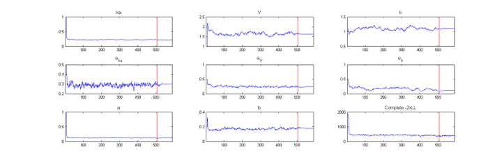
| − | The figure below displays the convergence of SAEM without simulated annealing to a local maximum of the likelihood (deviance = $-2\,\log {\like} | + | The figure below displays the convergence of SAEM without simulated annealing to a local maximum of the likelihood (deviance = $-2\,\log {\like} =816$). The initial values of the population parameters we chose were $(ka_0,V_0,k_0) = (1,1,1)$. |
{{ImageWithCaption|image=recuit1.png|size=720px|caption=Convergence of SAEM to a local maxima of the likelihood}} | {{ImageWithCaption|image=recuit1.png|size=720px|caption=Convergence of SAEM to a local maxima of the likelihood}} | ||
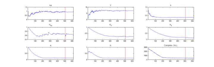
| − | Using the same initial guess, the | + | Using the same initial guess, the simulated annealing version of SAEM converges to the global maximum of the likelihood (deviance = 734). |
{{ImageWithCaption|image=recuit2.png|size=720px|caption=Convergence of SAEM to the global maxima of the likelihood }} | {{ImageWithCaption|image=recuit2.png|size=720px|caption=Convergence of SAEM to the global maxima of the likelihood }} | ||
Revision as of 16:33, 17 May 2013
Contents
Introduction
The SAEM (Stochastic Approximation of EM) algorithm is a stochastic algorithm for calculating the maximum likelihood estimator (MLE) in the quite general setting of incomplete data models. SAEM has been shown to be a very powerful NLMEM tool, known to accurately estimate population parameters as well as having good theoretical properties. In fact, it converges to the MLE under very general hypotheses.
SAEM was first implemented in the $\monolix$ software. It has also been implemented in NONMEM, the R package saemix and the Matlab statistics toolbox as the function nlmefitsa.m.
Here, we consider a model that includes observations $\by=(y_i , 1\leq i \leq N)$, unobserved individual parameters $\bpsi=(\psi_i , 1\leq i \leq N)$ and a vector of parameters $\theta$. By definition, the maximum likelihood estimator of $\theta$ maximizes
SAEM is an iterative algorithm that essentially consists of constructing $N$ Markov chains $(\psi_1^{(k)})$, ..., $(\psi_N^{(k)})$ that converge to the conditional distributions $\pmacro(\psi_1|y_1),\ldots , \pmacro(\psi_N|y_N)$, using at each step the complete data $(\by,\bpsi^{(k)})$ to calculate a new parameter vector $\theta_k$. We will present a general description of the algorithm highlighting the connection with the EM algorithm, and present by way of a simple example how to implement SAEM and use it in practice.
We will also give some extensions of the base algorithm that allow us to improve the convergence properties of the algorithm. For instance, it is possible to stabilize the algorithm's convergence by using several Markov chains per individual. Also, a simulated annealing version of SAEM allows us improve the chances of converging to the global maximum of the likelihood rather than to local maxima.
The EM algorithm
We first remark that if the individual parameters $\bpsi=(\psi_i)$ are observed, estimation is not thwarted by any particular problem because an estimator could be found by directly maximizing the joint distribution $\pypsi(\by,\bpsi ; \theta) $.
However, since the $\psi_i$ are not observed, the EM algorithm replaces $\bpsi$ by its conditional expectation. Then, given some initial value $\theta_0$, iteration $k$ updates ${\theta}_{k-1}$ to ${\theta}_{k}$ with the two following steps:
- $\textbf{E-step:}$ evaluate the quantity
- $\textbf{M-step:}$ update the estimation of $\theta$:
In can be proved that each EM iteration increases the likelihood of observations and that the EM sequence $(\theta_k)$ converges to a
stationary point of the observed likelihood under mild regularity conditions.
Unfortunately, in the framework of nonlinear mixed-effects models, there is no explicit expression for the E-step since the relationship between observations $\by$ and individual parameters $\bpsi$ is nonlinear. However, even though this expectation cannot be computed in a closed-form, it can be approximated by simulation. For instance,
- The Monte Carlo EM (MCEM) algorithm replaces the E-step by a Monte Carlo approximation based on a large number of independent simulations of the non-observed individual parameters $\bpsi$.
- The SAEM algorithm replaces the E-step by a stochastic approximation based on a single simulation of $\bpsi$.
The SAEM algorithm
At iteration $k$ of SAEM:
- $\textbf{Simulation step}$: for $i=1,2,\ldots, N$, draw $\psi_i^{(k)}$ from the conditional distribution $\pmacro(\psi_i |y_i ;\theta_{k-1})$.
- $\textbf{Stochastic approximation}$: update $Q_k(\theta)$ according to
where $(\gamma_k)$ is a decreasing sequence of positive numbers such that $\gamma_1=1$, $ \sum_{k=1}^{\infty} \gamma_k = \infty$ and $\sum_{k=1}^{\infty} \gamma_k^2 < \infty$.
- $\textbf{Maximization step}$: update $\theta_{k-1}$ according to
Implementation of SAEM is simplified when the complete model $\pmacro(\by,\bpsi;\theta)$ belongs to a regular (curved) exponential family:
where $\tilde{S}(\by,\bpsi)$ is a sufficient statistic of the complete model (i.e., whose value contains all the information needed to compute any estimate of $\theta$) which takes its values in an open subset ${\cal S}$ of $\Rset^m$. Then, there exists a function $\tilde{\theta}$ such that for any $s\in {\cal S}$,
\(
\tilde{\theta}(s) = \argmax{\theta} \left\{ - \zeta(\theta) + \langle s , \varphi(\theta) \rangle \right\} .
\)
|
(1) |
The approximation step of SAEM simplifies to a general Robbins-Monro-type scheme for approximating this conditional expectation:
- $\textbf{Stochastic approximation}$: update $s_k$ according to
Note that the E-step of EM simplifies to computing $s_k=\esp{\tilde{S}(\by,\bpsi) | \by ; \theta_{k-1}}$.
Then, both EM and SAEM algorithms use (1) for the M-step: $\theta_k = \tilde{\theta}(s_k)$.
Precise results for convergence of SAEM were obtained in (???) in the case where $\pmacro(\by,\bpsi;\theta)$ belongs to a regular curved exponential family. This first version of SAEM and these first results assume that the individual parameters are simulated exactly under the conditional distribution at each iteration. Unfortunately, for most nonlinear models or non-Gaussian models, the unobserved data cannot be simulated exactly under this conditional distribution. A well-known alternative consists in using the Metropolis-Hastings algorithm: introduce a transition probability which has as unique invariant distribution the conditional distribution we want to simulate.
In other words, the procedure consists of replacing the Simulation step of SAEM at iteration $k$ by $m$ iterations of the Metropolis-Hastings (MH) algorithm described in The Metropolis-Hastings algorithm section. It was shown in (???) that SAEM still converges under general conditions when coupled with a Markov chain Monte Carlo procedure.
Implementing SAEM
Implementation of SAEM can be difficult to describe when looking at complex statistical models such as mixture models, models with inter-occasion variability, etc. We are therefore going to limit ourselves to looking at some basic models in order to illustrate how SAEM can be implemented.
SAEM for a general hierarchical model
Consider first a very general model for any type (continuous, categorical, survival, etc.) of data $(y_i)$:
where $h(\psi_i)=(h_1(\psi_{i,1}), h_2(\psi_{i,2}), \ldots , h_d(\psi_{i,d}) )^\transpose$ is a $d$-vector of (transformed) individual parameters, $\mu$ a $d$-vector of fixed effects and $\Omega$ a $d\times d$ variance-covariance matrix.
We assume here that $\Omega$ is positive-definite. Then, a sufficient statistic for the complete model $\pmacro(\by,\bpsi;\theta)$ is $\tilde{S}(\bpsi) = (\tilde{S}_1(\bpsi),\tilde{S}_2(\bpsi))$, where
At iteration $k$ of SAEM, we have:
- $\textbf{Simulation step}$: for $i=1,2,\ldots, N$, draw $\psi_i^{(k)}$ from $m$ iterations of the MH algorithm described in The Metropolis-Hastings algorithm with $\pmacro(\psi_i |y_i ;\mu_{k-1},\Omega_{k-1})$ as limiting distribution.
- $\textbf{Stochastic approximation}$: update $s_k=(s_{k,1},s_{k,2})$ according to
- $\textbf{Maximization step}$: update $(\mu_{k-1},\Omega_{k-1})$ according to
What is remarkable is that it suffices to be able to calculate $\pcyipsii(y_i | \psi_i)$ for all $\psi_i$ and $y_i$ in order to be able to run SAEM. In effect, this allows the simulation step to be run using MH since the acceptance probabilities can be calculated.
SAEM for a continuous data model
Consider now a continuous data model in which the residual error variance is now constant:
Here, the individual parameters are $\psi_i=(\phi_i,a)$. The variance-covariance matrix for $\psi_i$ is not positive-definite in this case because $a$ has no variability. If we suppose that the variance matrix $\Omega$ is positive-definite, then noting $\theta=(\mu,\Omega,a)$, a natural decomposition of the model is:
The previous statistic $\tilde{S}(\bpsi) = (\tilde{S}_1(\bpsi),\tilde{S}_2(\bpsi))$ is not sufficient for estimating $a$. Indeed, we need an additional component which is a function both of $\by$ and $\bpsi$:
Then,
The choice of step-size $(\gamma_k)$ is extremely important for ensuring convergence of SAEM. The sequence $(\gamma_k)$ used in \monolix decreases like $k^{-\alpha}$. We recommend using $\alpha=0$ (that is, $\gamma_k=1$) during the first $K_1$ iterations, in order to converge quickly to a neighborhood of a maximum of the likelihood, and $\alpha=1$ during the next $K_2$ iterations. Indeed, the initial guess $\theta_0$ may be far from the maximum likelihood value we are looking for, and the first iterations with $\gamma_k=1$ allow SAEM to converge quickly to a neighborhood of this value. Following this, smaller step-sizes ensure the almost sure convergence of the algorithm to the maximum likelihood estimator.


A simple example to understand why SAEM converges in practice
Let us look at a very simple Gaussian model, with only one observation per individual:
We will furthermore assume that both $\omega^2$ and $\sigma^2$ are known.
Here, the maximum likelihood estimator $ \hat{\theta}$ of $\theta$ is easy to compute since $y_i \sim_{i.i.d.} {\cal N}(\theta,\omega^2+\sigma^2)$. We find that
We now propose to try and compute $\hat{\theta}$ using SAEM instead. The simulation step is straightforward since the conditional distribution of $\psi_i$ is a normal distribution:
where
The maximization step is also straightforward. Indeed, a sufficient statistics for estimating $\theta$ is
Then,
Let us first look at the behavior of SAEM when $\gamma_k=1$. At iteration $k$,
- Simulation step: $\psi_i^{(k)} \sim {\cal N}( a \theta_{k-1} + (1-a)y_i , \gamma^2). $
- Maximization step: $\theta_k = \displaystyle{ \frac{ {\cal S}(\bpsi^{(k)})}{N} } = \displaystyle{ \frac{1}{N} }\sum_{i=1}^{N} \psi_i^{(k)}$.
It can be shown that:
where $e_k \sim {\cal N}(0, \gamma^2 /N)$. Then, the sequence $(\theta_k)$ is an autoregressive process of order 1 (AR(1)) which converges in distribution to a normal distribution when $k\to \infty$:
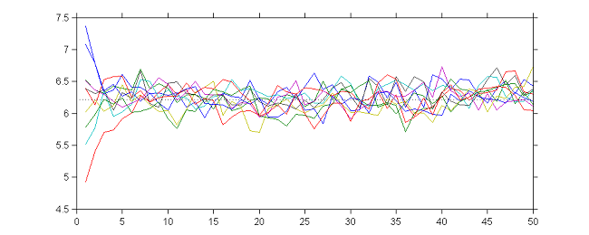 |
10 sequences $(\theta_k)$ obtained with different initial values and $\gamma_k=1$ for $1\leq k \leq 50$
|
Now, let us see what happens instead when $\gamma_k$ decreases like $1/k$. At iteration $k$,
- Simulation step: $\psi_i^{(k)} \sim {\cal N}( a \theta_{k-1} + (1-a)y_i , \gamma^2) $
- Maximization step:
- Here, we can show that:
- where $e_k \sim {\cal N}(0, \gamma^2 /N)$. Then, the sequence $(\theta_k)$ converges almost surely to $\hat{\theta}$.
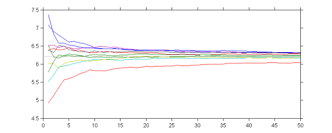 |
10 sequences $(\theta_k)$ obtained with different initial values and $\gamma_k=1/k$ for $1\leq k \leq 50$
|
Thus, we see that by combining the two strategies, the sequence $(\theta_k)$ is a Markov chain that converges to a random walk around $\hat{\theta}$ during the first $K_1$ iterations, then converges almost surely to $\hat{\theta}$ during the next $K_2$ iterations.
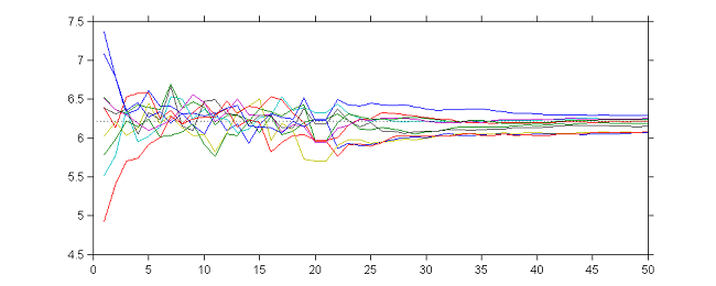 |
10 sequences $(\theta_k)$ obtained with different initial values, $\gamma_k=1$ for $1\leq k \leq 20$ and $\gamma_k=1/(k-20)$ for $21\leq k \leq 50$
|
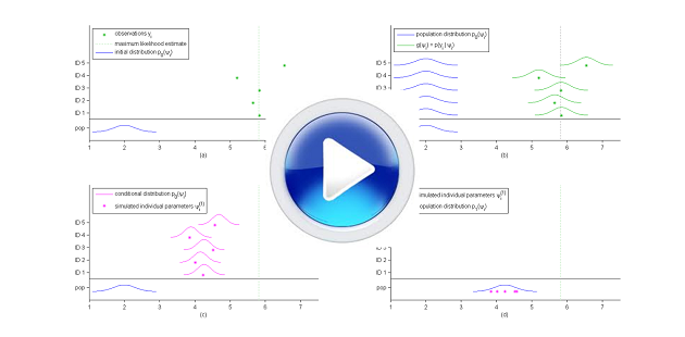
The SAEM algorithm in practice.
|
A simulated annealing version of SAEM
Convergence of SAEM can strongly depend on the initial guess when the likelihood ${\like}$ has several local maxima. A simulated annealing version of SAEM can improve convergence of the algorithm toward the global maximum of ${\like}$.
To detail this, we can first rewrite the joint pdf of $(\by,\bpsi)$ as follows:
where $C(\theta)$ is a normalizing constant that only depends on $\theta$.
Then, for any "temperature" $T\geq0$, we consider the complete model
where $C_T(\theta)$ is still a normalizing constant.
We then introduce a decreasing temperature sequence $(T_k, 1\leq k \leq K)$ and use the SAEM algorithm on the complete model $\pmacro_{T_k}(\by,\bpsi;\theta)$ at iteration $k$ (the usual version of SAEM uses $T_k=1$ at each iteration). The sequence $(T_k)$ is chosen to have large positive values during the first iterations, then decrease with an exponential rate to 1: $ T_k = \max(1, \tau \ T_{k-1}) $.
Consider for example the following model for continuous data:
Here, $\theta = (\mu,\Omega,a^2)$ and
where $C(\theta)$ is a normalizing constant that only depends on $a$ and $\Omega$.
We see that $\pmacro_T(\by,\bpsi;\theta)$ will also be a normal distribution whose residual error variance $a^2$ is replaced by $T a^2$ and variance matrix $\Omega$ for the random effects by $T\Omega$.
In other words, a model with a "large temperature" is a model with large variances.
The algorithm therefore consists in choosing large initial variances $\Omega_0$ and $a^2_0$ (that include the initial temperature $T_0$ implicitly) and setting $ a^2_k = \max(\tau \ a^2_{k-1} , \hat{a}(\by,\bpsi^{(k)}) $ and $ \Omega_k = \max(\tau \ \Omega_{k-1} , \hat{\Omega}(\bpsi^{(k)}) $ during the first iterations. Here, $0\leq\tau\leq 1$.
These large values of the variance make the conditional distributions $\pmacro_T(\psi_i | y_i;\theta)$ less concentrated around their modes, and thus allows the sequence $(\theta_k)$ to "escape" from local maxima of the likelihood during the first iterations of SAEM and converge to a neighborhood of the global maximum of ${\like}$. After these initial iterations, the usual SAEM algorithm is used to estimate these variances at each iteration.
 |
 |