Estimation

Introduction

In the modeling context, we usually assume that we have data that includes observations $\by$, measurement times $\bt$ and possibly additional regression variables $\bx$. There may also be individual covariates $\bc$, and in pharmacological applications the dose regimen $\bu$. For clarity, in the following notation we will omit the design variables $\bt$, $\bx$ and $\bu$, and the covariates $\bc$.

Here, we find ourselves in the classical framework of incomplete data models. Indeed, only $\by = (y_{ij})$ is observed in the joint model $\pypsi(\by,\bpsi;\theta)$.

Estimation tasks are common ones seen in statistics:

Estimate the population parameter $\theta$ using the available observations and possibly a priori information that is available.
Evaluate the precision of the proposed estimates.
Reconstruct missing data, here being the individual parameters $\bpsi=(\psi_i, 1\leq i \leq N)$.
Estimate the log-likelihood for a given model, i.e., for a given joint distribution $\qypsi$ and value of $\theta$.

Maximum likelihood estimation of the population parameters

Definitions

Maximum likelihood estimation consists of maximizing with respect to $\theta$ the observed likelihood defined by:

$\begin{eqnarray} \like(\theta ; \by) &\eqdef& \py(\by ; \theta) \\ &=& \int \pypsi(\by,\bpsi ;\theta) \, d \bpsi . \end{eqnarray}$

Maximum likelihood estimation of the population parameter $\theta$ requires:

A model, i.e., a joint distribution $\qypsi$. Depending on the software used, the model can be implemented using a script or a graphical user interface. $\monolix$ is extremely flexible and allows us to combine both. It is possible for instance to code the structural model using $\mlxtran$ and use the GUI for implementing the statistical model. Whatever the options selected, the complete model can always be saved as a text file.

Inputs $\by$, $\bc$, $\bu$ and $\bt$. All of these variables tend to be stored in a unique data file (see the Data Exploration Section).

An algorithm which allows us to maximize $\int \pypsi(\by,\bpsi ;\theta) \, d \bpsi$ with respect to $\theta$. Each software package has its own algorithms implemented. It is not our goal here to rate and compare the various algorithms and implementations. We will use exclusively the SAEM algorithm as described in The SAEM algorithm and implemented in $\monolix$ as we are entirely satisfied by both its theoretical and practical qualities:

The algorithms implemented in $\monolix$ including SAEM and its extensions (mixture models, hidden Markov models, SDE-based model, censored data, etc.) have been published in statistical journals. Furthermore, convergence of SAEM has been rigorously proved.

The SAEM implementation in $\monolix$ is extremely efficient for a wide variety of complex models.

The SAEM implementation in $\monolix$ was done by the same group that proposed the algorithm and studied in detail its theoretical and practical properties.

Remark

It is important to highlight the fact that for a parameter $\psi_i$ whose distribution is the transformation of a normal one (log-normal, logit-normal, etc.) the MLE $\hat{\psi}_{\rm pop}$ of the reference parameter $\psi_{\rm pop}$ is neither the mean nor the mode of the distribution. It is in fact the median.

To show why this is the case, let $h$ be a nonlinear, twice continuously derivable and strictly increasing function such that $h(\psi_i)$ is normally distributed.

First we show that it is not the mean. By definition, the MLE of $h(\psi_{\rm pop})$ is $h(\hat{\psi}_{\rm pop})$. Thus, the estimated distribution of $h(\psi_i)$ is the normal distribution with mean $h(\hat{\psi}_{\rm pop})$, but $\esp{h(\psi_i)} = h(\hat{\psi}_{\rm pop})$ implies that $\esp{\psi_i} \neq \hat{\psi}_{\rm pop}$ since $h$ is nonlinear. In other words, $\hat{\psi}_{\rm pop}$ is not the mean of the estimated distribution of $\psi_i$.

Next we show that it is not the mode. Let $f$ be the pdf of $\psi_i$ and let $f_h$ be the pdf of $h(\psi_i)$. By definition, for any $h(t)\in \mathbb{R}$,

$ f(t) = h^\prime(t)f_h(h(t)) . $

Thus,

$ f^\prime(t) = h^{\prime \prime}(t)f_h(h(t)) + h^{\prime 2}(t)f_h^\prime(h(t)) . $

By definition of the mode, $f_h^\prime(h(\hat{\psi}_{\rm pop}))=0$. Since $h$ is nonlinear, $h^{\prime \prime}(\hat{\psi}_{\rm pop})\neq 0$ a.s. and $f^\prime(\hat{\psi}_{\rm pop})\neq 0$ a.s.. In other words, $\hat{\psi}_{\rm pop}$ is not the mode of the estimated distribution of $\psi_i$.

Now we show that it is the median. Since $h$ is a strictly increasing function,

$\begin{eqnarray} \probs{\hat{\psi}_{\rm pop} }{\psi_i \leq \hat{\psi}_{\rm pop} } &=& \probs{\hat{\psi}_{\rm pop} }{h(\psi_i) \leq h(\hat{\psi}_{\rm pop})} \\ &=& 0.5 . \end{eqnarray}$

In other words, $\hat{\psi}_{\rm pop}$ is the median of the estimated distribution of $\psi_i$.

Example

Let us again look at the model used in the Model Visualization Section. For the case of a unique dose $D$ given at time $t=0$, the structural model is written:

$\begin{eqnarray} ke&=&Cl/V \\ Cc(t) &=& \displaystyle{\frac{D \, ka}{V(ka-ke)} }\left(e^{-ke\,t} - e^{-ka\,t} \right) \\ h(t) &=& h_0 \, \exp(\gamma\, Cc(t)) , \end{eqnarray}$

where $Cc$ is the concentration in the central compartment and $h$ the hazard function for the event of interest (hemorrhaging). Supposing a constant error model for the concentration, the model for the observations can be easily implemented using $\mlxtran$.

MLXTran  joint1est_model.txt

 
INPUT:
parameter =  {ka, V, Cl, h0, gamma}

EQUATION:
ke=Cl/V
Cc  = amtDose*ka/(V*(ka-ke))*(exp(-ke*t) - exp(-ka*t))
h = h0*exp(gamma*Cc)

OBSERVATION:
Concentration = {type=continuous, prediction=Cc, errorModel=constant}
Hemorrhaging  = {type=event, hazard=h}

OUTPUT:
output = {Concentration, Hemorrhaging}

Here, amtDose is a reserved keyword for the last administered dose.

The model's parameters are the absorption rate constant $ka$, the volume of distribution $V$, the clearance $Cl$, the baseline hazard $h_0$ and the coefficient $\gamma$. The statistical model for the individual parameters can be defined in the $\monolix$ project file (left) and/or the $\monolix$ GUI (right):

MLXTran   

 
INDIVIDUAL:
     ka    = {distribution=logNormal, iiv=yes}
     V     = {distribution=logNormal, iiv=yes},
     Cl    = {distribution=normal, iiv=yes},
     h0    = {distribution=probitNormal, iiv=yes},
     gamma = {distribution=logitNormal, iiv=yes},

Once the model is implemented, tasks such as maximum likelihood estimation can be performed using the SAEM algorithm. Certain settings in SAEM must be provided by the user. Even though SAEM is quite insensitive to the initial parameter values, it is possible to perform a preliminary sensitivity analysis in order to select "good" initial values.

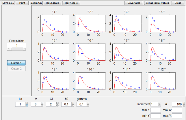Looking for good initial values for SAEM

Then, when we run SAEM, it converges easily and quickly to the MLE:

Estimation of the population parameters

              parameter
ka          :    0.974
V           :     7.07
Cl          :     2.00
h0          :   0.0102
gamma       :    0.485

omega_ka    :    0.668
omega_V     :    0.365
omega_Cl    :    0.588
omega_h0    :    0.105
omega_gamma :   0.0901

a_1         :    0.345

Parameter estimation can therefore be seen as estimating the reference values and variance of the random effects.

In addition to these numbers, it is important to be able to graphically represent these distributions in order to see them and therefore understand them better. In effect, the interpretation of certain parameters is not always simple. Of course, we know what a normal distribution represents and in particular its mean, median and mode, which are equal (see the distribution of $Cl$ below for instance). These measures of central tendency can be different among themselves for other asymmetric distributions such as the log-normal (see the distribution of $ka$).

Interpreting dispersion terms like $\omega_{ka}$ and $\omega_{V}$ is not obvious either when the parameter distributions are not normal. In such cases, quartiles or quantiles of order 5% and 95% (for example) may be useful for quantitively describing the variability of these parameters.

Remarks

For a parameter $\psi$ whose distribution is log-normal, we can approximate the coefficient of variation for $\psi$ by the standard deviation $\omega_{\psi}$ of the random effect $\eta$ if this is fairly small. In effect, when $\omega_{\psi}$ is small,

$\begin{eqnarray} \psi &=& \psi_{\rm pop} e^{\eta} \\ &\approx & \psi_{\rm pop}(1+ \eta) . \end{eqnarray}$

Thus

$\begin{eqnarray} \esp{\psi} &\approx& \psi_{\rm pop} \\ \std{\psi} &\approx & \psi_{\rm pop}\omega_{\psi}, \end{eqnarray}$

and

$\begin{eqnarray} {\rm cv}(\psi) &=& \frac{\std{\psi} }{\esp{\psi} } \\ &\approx & \omega_{\psi} . \end{eqnarray}$

Do not forget that this approximation is only valid when $\omega$ is small and in the case of log-normal distributions. It does not carry over to any other distribution. Thus, when $\omega_{h0}=0.1$ for a probit-normal distribution or $\omega_{\gamma}=0.09$ for a logit-normal one, there is no immediate interpretation available. Only by looking at the graphical display of the pdf or by calculating some quantiles of interest can we begin to get an idea of dispersion in the parameters $h0$ and $\gamma$.

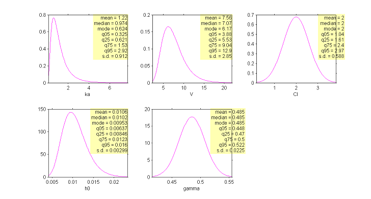Estimation of the population distributions of the individual parameters of the model

Bayesian estimation of the population parameters

The Bayesian approach considers $\theta$ as a random vector with a prior distribution $\qth$. We can then define the posterior distribution of $\theta$:

$\begin{eqnarray} \pcthy(\theta | \by ) &=& \displaystyle{ \frac{\pth( \theta )\pcyth(\by | \theta )}{\py(\by)} }\\ &=& \displaystyle{ \frac{\pth( \theta ) \int \pypsith(\by,\bpsi |\theta) \, d \bpsi}{\py(\by)} }. \end{eqnarray}$

We can estimate this conditional distribution and derive any statistics (posterior mean, standard deviation, percentiles, etc.) or derive the so-called Maximum a Posteriori (MAP) estimate of $\theta$:

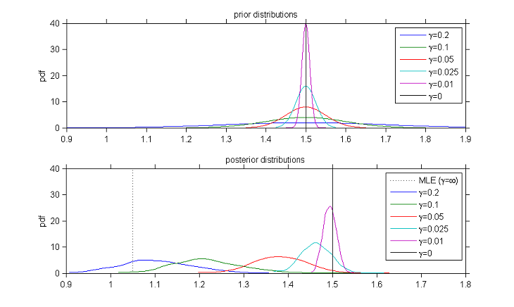
$\begin{eqnarray} \hat{\theta}^{\rm MAP} &=& \argmax{\theta} \pcthy(\theta | \by ) \\ &=& \argmax{\theta} \left\{ {\llike}(\theta ; \by) + \log( \pth( \theta ) ) \right\} . \end{eqnarray}$

The MAP estimate therefore maximizes a penalized version of the observed likelihood. In other words, maximum a posteriori estimation reduces to penalized maximum likelihood estimation. Suppose for instance that $\theta$ is a scalar parameter and the prior is a normal distribution with mean $\theta_0$ and variance $\gamma^2$. Then, the MAP estimate minimizes

$ \hat{\theta}^{\rm MAP} =\argmax{\theta} \left\{ {\llike} (\theta ; \by) - \displaystyle{ \frac{1}{2\gamma^2} }(\theta - \theta_0)^2 \right\} . $

The MAP estimate is a trade-off between the MLE which maximizes ${\llike}(\theta ; \by)$ and $\theta_0$ which minimizes $(\theta - \theta_0)^2$. The weight given to the prior directly depends on the variance of the prior distribution: the smaller $\gamma^2$ is, the closer to $\theta_0$ the MAP is. The limiting distribution considers that $\gamma^2=0$: this prior means here that $\theta$ is fixed as $\theta_0$ and no longer needs to be estimated.

Both the Bayesian and frequentist approaches have their supporters and detractors. But rather than being dogmatic and blindly following the same rule-book every time, we need to be pragmatic and ask the right methodological questions when confronted with a new problem.

We have to remember that Bayesian methods have been extremely successful, in particular for numerical calculations. For instance, (Bayesian) MCMC methods allow us to estimate more or less any conditional distribution coming from any hierarchical model, whereas frequentist approaches such as maximum likelihood estimation can be much more difficult to implement.

All things said, the problem comes down to knowing whether the data contains sufficient information to answer a given question, and whether some other information may be available to help answer it. This is the essence of the art of modeling: finding the right compromise between the confidence we have in the data and prior knowledge of the problem. Each problem is different and requires a specific approach. For instance, if all the patients in a pharmacokinetic trial have essentially the same weight, it is pointless to estimate a relationship between weight and the model's PK parameters using the trial data. In this case, the modeler would be better served trying to use prior information based on physiological criteria rather than just a statistical model.

Therefore, we can use information available to us, of course! Why not? But this information needs to be pertinent. Systematically using a prior for the parameters is not always meaningful. Can we reasonable suppose that we have access to such information? For continuous data for example, what does putting a prior on the residual error model's parameters mean in reality? A reasoned statistical approach consists of only including prior information for certain parameters (those for which we have real prior information) and having confidence in the data for the others.

$\monolix$ allows this hybrid approach which reconciles the Bayesian and frequentist approaches. A given parameter can be:

a fixed constant if we have absolute confidence in its value or the data does not allow it to be estimated, essentially due to identifiability constraints.

estimated by maximum likelihood, either because we have great confidence in the data or have no information on the parameter.

estimated by introducing a prior and calculating the MAP estimate.

estimated by introducing a prior and then estimating the posterior distribution.

We put aside dealing with the fixed components of $\theta$ in the following. Here are some possible situations:

Combined maximum likelihood and maximum a posteriori estimation: decompose $\theta$ into $(\theta_E,\theta_{M})$ where $\theta_E$ are the components of $\theta$ to be estimated with MLE and $\theta_{M}$ those with a prior distribution whose posterior distribution is to be maximized. Then, $(\hat{\theta}_E , \hat{\theta}_{M} )$ below maximizes the penalized likelihood of $(\theta_E,\theta_{M})$:

$\begin{eqnarray} (\hat{\theta}_E , \hat{\theta}_{M} ) &=& \argmax{\theta_E , \theta_{M} } \log(\py(\by , \theta_{M}; \theta_E)) \\ &=& \argmax{\theta_E , \theta_{M} } \left\{ {\llike}(\theta_E , \theta_{M}; \by) + \log( \pth( \theta_M ) ) \right\} , \end{eqnarray}$

where ${\llike} (\theta_E , \theta_{M}; \by) \ \ \eqdef \ \ \log\left(\py(\by | \theta_{M}; \theta_E)\right).$

Combined maximum likelihood and posterior distribution estimation: here, decompose $\theta$ into $(\theta_E,\theta_{R})$ where $\theta_E$ are the components of $\theta$ to be estimated with MLE and $\theta_{R}$ those with a prior distribution whose posterior distribution is to be estimated. We propose the following strategy for estimating $\theta_E$ and $\theta_{R}$:

Compute the maximum likelihood of $\theta_E$:

$\begin{eqnarray} \hat{\theta}_E &=& \argmax{\theta_E} \log(\py(\by ; \theta_E)) \\ &=& \argmax{\theta_E} \int \pmacro(\by , \theta_R ; \theta_E ) d \theta_R . \end{eqnarray}$

Estimate the conditional distribution $\pmacro(\theta_{R} | \by ;\hat{\theta}_E)$.

It is then straightforward to extend this approach to more complex situations where some components of $\theta$ are estimated with MLE, others using MAP estimation and others still by estimating their conditional distributions.

Example A PK example

In this example we use only the pharmacokinetic data and aim to estimate the population parameter distributions of the PK parameters $ka$, $V$ and $Cl$. We assume log-normal distributions for these three parameters. All of the model's population parameters are estimated by maximum likelihood estimation except $ka_{\rm pop}$ for which a log-normal distribution is used as a prior:

$ \log(ka_{\rm pop}) \sim {\cal N}(\log(1.5), \gamma^2) . $

$\monolix$ allows us to compute the MAP estimate and to estimate the posterior distribution of $ka_{\rm pop}$ for various values of $\gamma$.

$\gamma$	0	0.01	0.025	0.05	0.1	0.2	$+ \infty$
$\hat{ka}_{\rm pop}^{\rm MAP}$	1.5	1.49	1.47	1.39	1.22	1.11	1.05

Prior and posterior distributions of $ka_{\rm pop}$ for different values of $\gamma$

As expected, the posterior distribution converges to the prior distribution when the standard deviation $\gamma$ of the prior distribution decreases. Also, the mode of the posterior distribution converges to the maximum likelihood estimate of $ka_{\rm pop}$ when $\gamma$ increases.

Estimation of the Fisher information matrix

The variance of the estimator $\thmle$ and thus confidence intervals can be derived from the observed Fisher information matrix (F.I.M.), which itself is calculated using the observed likelihood (i.e., the pdf of the observations $\by$):

$ \ofim(\thmle ; \by) \ \ \eqdef \ \ - \displaystyle{ \frac{\partial^2}{\partial \theta^2} }\log({\like}(\thmle ; \by)) . $

(1)

Then, the variance-covariance matrix of the maximum likelihood estimator $\thmle$ can be estimated by the inverse of the observed F.I.M. Standard errors (s.e.) for each component of $\thmle$ are their standard deviations, i.e., the square-root of the diagonal elements of this covariance matrix. $\monolix$ also displays the (estimated) relative standard errors (r.s.e.), i.e., the (estimated) standard error divided by the value of the estimated parameter.

Estimation of the population parameters

              parameter     s.e. (s.a.)   r.s.e.(%)
ka          :    0.974         0.082           8
V           :     7.07          0.35           5
Cl          :        2          0.07           4
h0          :   0.0102        0.0014          14
gamma       :    0.485         0.015           3

omega_ka    :    0.668         0.064          10
omega_V     :    0.365         0.037          10
omega_Cl    :    0.588         0.055           9
omega_h0    :    0.105         0.032          30
omega_gamma :   0.0901         0.044          49

a_1         :    0.345         0.012           3

The F.I.M. can be used for detecting overparametrization of the structural model. In effect, if the model is poorly identifiable, certain estimators will be quite correlated and the F.I.M. will therefore be poorly conditioned and difficult to inverse. Suppose for example that we want to fit a two compartment PK model to the same data as before. The output is shown below. The large values for the relative standard errors for the inter-compartmental clearance $Q$ and the volume of the peripheral compartment $V_2$ mean that the data does not allow us to estimate well these two parameters.

Estimation of the population parameters

           parameter     s.e. (lin)   r.s.e.(%)
ka       :     0.246       0.0081             3
Cl       :       1.9        0.075             4
V1       :      1.71         0.14             8
Q        :  0.000171        0.024      1.43e+04
V2       :   0.00673          3.1      4.62e+04

omega_ka :     0.171        0.026            15
omega_Cl :     0.293        0.026             9
omega_V1 :     0.621        0.062            10
omega_Q  :      5.72      1.4e+03      2.41e+04
omega_V2 :      4.61      1.8e+04      3.94e+05

a        :     0.136       0.0073             5

The Fisher information criteria is also widely used in optimal experimental design. Indeed, minimizing the variance of the estimator corresponds to maximizing the information. Then, estimators and designs can be evaluated by looking at certain summary statistics of the covariance matrix (like the determinant or trace for instance).

Estimation of the individual parameters

Once $\theta$ has been estimated, the conditional distribution $\pmacro(\psi_i | y_i ; \hat{\theta})$ of the individual parameters $\psi_i$ can be estimated for each individual $i$ using the Metropolis-Hastings algorithm. For each $i$, this algorithm generates a sequence $(\psi_i^{k}, k \geq 1)$ which converges in distribution to the conditional distribution $\pmacro(\psi_i | y_i ; \hat{\theta})$ and that can be used for estimating any summary statistic of this distribution (mean, standard deviation, quantiles, etc.).

The mode of this conditional distribution can be estimated using this sequence or by maximizing $\pmacro(\psi_i | y_i ; \hat{\theta})$ using numerical methods.

The choice of using the conditional mean or the conditional mode is arbitrary. By default, $\monolix$ uses the conditional mode, taking the philosophy that the "most likely" values of the individual parameters are the most suited for computing the "most likely" predictions.

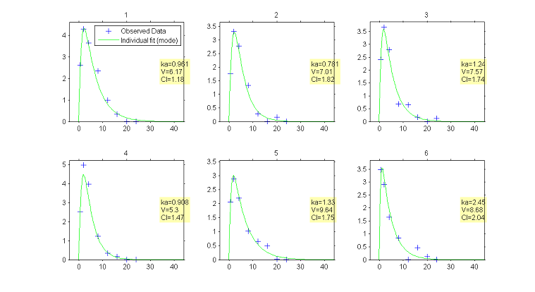Predicted concentrations for 6 individuals using the estimated conditional modes of the individual PK parameters

Estimation of the observed log-likelihood

Once $\theta$ has been estimated, the observed log-likelihood of $\hat{\theta}$ is defined as

$ \begin{eqnarray} {\llike} (\hat{\theta};\by) &=& \log({\like}(\hat{\theta};\by)) \\ &\eqdef& \log(\py(\by;\hat{\theta})) . \end{eqnarray}$

The observed log-likelihood cannot be computed in closed form for nonlinear mixed effects models, but can be estimated using the methods described in the Estimation of the log-likelihood Section. The estimated log-likelihood can then be used for performing likelihood ratio tests and for computing information criteria such as AIC and BIC (see the Model evaluation Section).

Bibliography

Lixoft - Monolix 4.2

http://www.lixoft.eu/products/monolix/product-monolix-overview ,2012

Bibtex

Author : Lixoft
Title : Monolix 4.2
In : http://www.lixoft.eu/products/monolix/product-monolix-overview -
Address :
Date : 2012

Comets, E., Lavenu, A., Lavielle, M. - saemix: Stochastic Approximation Expectation Maximization (SAEM) algorithm. R package version 0.96.1

http://cran.r-project.org/web/packages/saemix/index.html ,2013

Bibtex

Author : Comets, E., Lavenu, A., Lavielle, M.
Title : saemix: Stochastic Approximation Expectation Maximization (SAEM) algorithm. R package version 0.96.1
In : http://cran.r-project.org/web/packages/saemix/index.html -
Address :
Date : 2013

The MathWorks - nlmefitsa: fit nonlinear mixed-effects model with stochastic EM algorithm. Matlab R2013a function

http://www.mathworks.fr/fr/help/stats/nlmefitsa.html ,2013

Bibtex

Author : The MathWorks
Title : nlmefitsa: fit nonlinear mixed-effects model with stochastic EM algorithm. Matlab R2013a function
In : http://www.mathworks.fr/fr/help/stats/nlmefitsa.html -
Address :
Date : 2013

Beal, S.L., Sheiner, L.B., Boeckmann, A., Bauer, R.J. - NONMEM users guides

San Francisco, NONMEM Project Group, University of California ,1992

Bibtex

Author : Beal, S.L., Sheiner, L.B., Boeckmann, A., Bauer, R.J.
Title : NONMEM users guides
In : San Francisco, NONMEM Project Group, University of California -
Address :
Date : 1992

Pinheiro, J.C., Bates, D.M. - Mixed effects models in S and S-PLUS

Springer Verlag,2000

Bibtex

Author : Pinheiro, J.C., Bates, D.M.
Title : Mixed effects models in S and S-PLUS
In : -
Address :
Date : 2000

Pinheiro, J., Bates, D., DebRoy, S., Sarkar, D. - the R Core team (2009) nlme: Linear and Nonlinear Mixed Effects Models. R package version 3.1-96

R Foundation for Statistical Computing, Vienna ,2010

Bibtex

Author : Pinheiro, J., Bates, D., DebRoy, S., Sarkar, D.
Title : the R Core team (2009) nlme: Linear and Nonlinear Mixed Effects Models. R package version 3.1-96
In : R Foundation for Statistical Computing, Vienna -
Address :
Date : 2010

Spiegelhalter, D., Thomas, A., Best, N., Lunn, D. - WinBUGS user manual

Cambridge: MRC Biostatistics Unit ,2003

Bibtex

Author : Spiegelhalter, D., Thomas, A., Best, N., Lunn, D.
Title : WinBUGS user manual
In : Cambridge: MRC Biostatistics Unit -
Address :
Date : 2003

SPSS - Linear mixed-effects modeling in SPSS. An introduction to the MIXED procedure

,2002

Bibtex

Author : SPSS
Title : Linear mixed-effects modeling in SPSS. An introduction to the MIXED procedure
In : -
Address :
Date : 2002

SAS - The NLMMIXED procedure, SAS/STAT 9.2 User's Guide