Difference between revisions of "Overview"
m |
m |
||
| Line 1: | Line 1: | ||
| − | + | The desire to model a biological or physical phenomenon often arises when we are able to record some observations issued from that phenomenon. Nothing would be more natural therefore than to begin this introduction by looking at some observed data. | |
{{ExampleWithImage | {{ExampleWithImage | ||
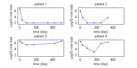
| − | |text= This first | + | |text= This first plot display the viral load of four patients with hepatitis C who started a treatment at time $t=0$. |
|image = NEWintro1.png | |image = NEWintro1.png | ||
}} | }} | ||
| Line 8: | Line 8: | ||
{{ExampleWithImage | {{ExampleWithImage | ||
| − | |text=This second example involves weight data | + | |text=This second example involves weight data for rats measured over 14 weeks, for a sub-chronic toxicity study related to the question of genetically modified corn. |
|image = NEWintro2.png}} | |image = NEWintro2.png}} | ||
{{ExampleWithImage | {{ExampleWithImage | ||
| − | |text= | + | |text= In this third example, data are fluorescence intensities measured over time in a cellular biology experiment. |
|image=NEWintro3.png }} | |image=NEWintro3.png }} | ||
{{ExampleWithImage | {{ExampleWithImage | ||
| − | |text= | + | |text= Note that repeated measurements are not necessarily always functions of time. |
| + | For example, we may be interested in corn production as a function of fertilizer quantity. | ||
|image= NEWintro4.png}} | |image= NEWintro4.png}} | ||
| + | Even though these examples come from quite different domains, in each case the data is made up of repeated measurements on several individuals from a population. What we will call a `"population approach'" is therefore relevant for characterizing and modeling this data. The modeling goal is thus twofold: characterize the biological or physical phenomena observed for each individual, and secondly, the variability seen between individuals. | ||
| + | |||
| + | In the example with the rats, the model needs to integrate a growth model that describes how a rat's weight increases with time, and a statistical model that describes why these kinetics can vary from one rat to another. The goal is thus to finish with a "typical'" curve for the population (in red) and to be able to explain the variability in the individual's curves (in green) around this population curve. | ||
| Line 27: | Line 31: | ||
| + | The model will explain some of this variability by individual covariates such as sex or diet (rats 1 and 3 are male while rats 2 and 4 are female), but some of the variability will remain unexplained and will be considered as random. Integrating into the same model effects considered fixed and others considered random leads naturally to the use of mixed-effects models. | ||
| + | |||
| + | An alternative yet equivalent approach considers this model as a hierarchical one: each curve is described by a single model, and the variability between individual models is described by a population model. In the case of parametric models, this means that the observations for a given individual are described by a model of the observations that depends on a vector of individual parameters: this is the classic individual approach. The population approach is then a direct extension of the individual approach: we add a component to the model that describes the variability of the individual parameters within the population. | ||
| + | |||
| + | A model can thus be seen as a joint probability distribution, which can easily be extended to the case where other variables in the model are considered as random variables: covariates, population parameters, the design, etc. The hierarchical structure of the model leads to a natural decomposition of the joint distribution into a product of conditional and marginal distributions. | ||
| + | |||
| + | Models for individual parameters and models for observations are described in the Models chapter. In particular, models for continuous observations, categorical, count and survival data are presented and illustrated by various examples. Extensions for mixture models, hidden Markov models and stochastic differential equation-based models are also presented. | ||
| + | |||
| + | The Tasks & Tools chapter presents practical examples of using these models: exploration and visualization, estimation, model diagnostics, model selection and simulation. All approaches and proposed methods are rigorously detailed in the Methods chapter. | ||
| + | The main purpose of a model is to be used. Mathematical modeling and statistics are useful tools in the service of many disciplines (biology, agronomy, environmental studies, pharmacology, etc.), but it is important that these tools are used properly. The various software packages used in this wiki have been developed with this in mind: they serve the modeler well, while fully complying with a coherent mathematical formalism and using well-known and theoretically justified methods. | ||
Revision as of 11:16, 4 June 2013
The desire to model a biological or physical phenomenon often arises when we are able to record some observations issued from that phenomenon. Nothing would be more natural therefore than to begin this introduction by looking at some observed data.
This first plot display the viral load of four patients with hepatitis C who started a treatment at time $t=0$.
|
|
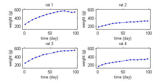
This second example involves weight data for rats measured over 14 weeks, for a sub-chronic toxicity study related to the question of genetically modified corn.
|
|
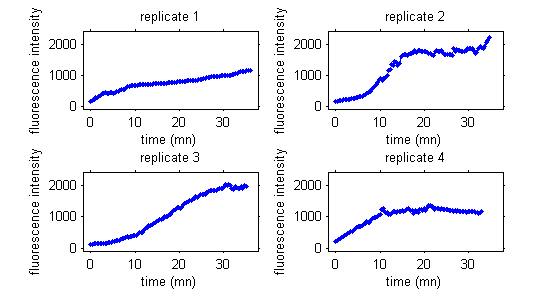
In this third example, data are fluorescence intensities measured over time in a cellular biology experiment.
|
|
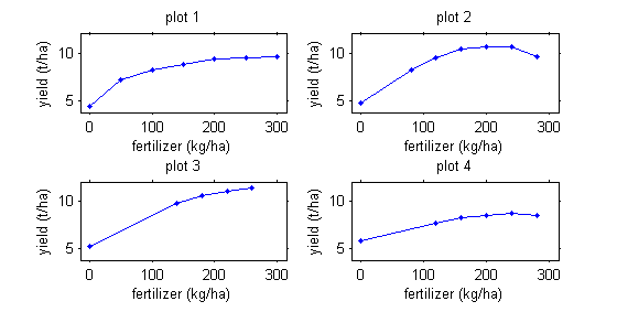
Note that repeated measurements are not necessarily always functions of time.
For example, we may be interested in corn production as a function of fertilizer quantity.
|
|
Even though these examples come from quite different domains, in each case the data is made up of repeated measurements on several individuals from a population. What we will call a `"population approach'" is therefore relevant for characterizing and modeling this data. The modeling goal is thus twofold: characterize the biological or physical phenomena observed for each individual, and secondly, the variability seen between individuals.
In the example with the rats, the model needs to integrate a growth model that describes how a rat's weight increases with time, and a statistical model that describes why these kinetics can vary from one rat to another. The goal is thus to finish with a "typical'" curve for the population (in red) and to be able to explain the variability in the individual's curves (in green) around this population curve.

The model will explain some of this variability by individual covariates such as sex or diet (rats 1 and 3 are male while rats 2 and 4 are female), but some of the variability will remain unexplained and will be considered as random. Integrating into the same model effects considered fixed and others considered random leads naturally to the use of mixed-effects models.
An alternative yet equivalent approach considers this model as a hierarchical one: each curve is described by a single model, and the variability between individual models is described by a population model. In the case of parametric models, this means that the observations for a given individual are described by a model of the observations that depends on a vector of individual parameters: this is the classic individual approach. The population approach is then a direct extension of the individual approach: we add a component to the model that describes the variability of the individual parameters within the population.
A model can thus be seen as a joint probability distribution, which can easily be extended to the case where other variables in the model are considered as random variables: covariates, population parameters, the design, etc. The hierarchical structure of the model leads to a natural decomposition of the joint distribution into a product of conditional and marginal distributions.
Models for individual parameters and models for observations are described in the Models chapter. In particular, models for continuous observations, categorical, count and survival data are presented and illustrated by various examples. Extensions for mixture models, hidden Markov models and stochastic differential equation-based models are also presented.
The Tasks & Tools chapter presents practical examples of using these models: exploration and visualization, estimation, model diagnostics, model selection and simulation. All approaches and proposed methods are rigorously detailed in the Methods chapter.
The main purpose of a model is to be used. Mathematical modeling and statistics are useful tools in the service of many disciplines (biology, agronomy, environmental studies, pharmacology, etc.), but it is important that these tools are used properly. The various software packages used in this wiki have been developed with this in mind: they serve the modeler well, while fully complying with a coherent mathematical formalism and using well-known and theoretically justified methods.
 |