Difference between revisions of "Introduction to PK modeling using MLXPlore - Part I"
m |
m |
||
| Line 1: | Line 1: | ||
| − | + | == Introduction == | |
| − | |||
| − | |||
| − | |||
This is an introductory tutorial for describing and visualizing simple and more complex pharmacokinetic (PK) models. | This is an introductory tutorial for describing and visualizing simple and more complex pharmacokinetic (PK) models. | ||
| Line 13: | Line 10: | ||
<br> | <br> | ||
| − | + | == Absorption == | |
| − | === | + | === First-order and zero-order absorption === |
| Line 38: | Line 35: | ||
<br> | <br> | ||
| − | === | + | === First-order, zero-order and $\alpha$-order absorption === |
| Line 59: | Line 56: | ||
<br> | <br> | ||
| − | === | + | === First-order, zero-order and sequential zero-order/first-order absorption === |
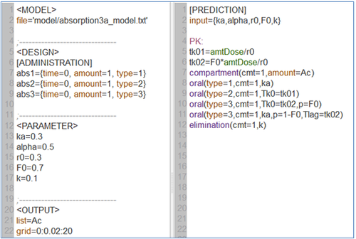
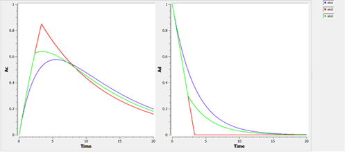
<span style="color:#993300">{{Verbatim|absorption3a_script :}}</span> we compute and display the amount in the central compartment when the drug is transferred from the depot to the central compartment with a first-order, zero-order or sequential zero-order/first-order absorption process. Here, $r0$ is the absorption rate for the zero-order process and $F0$ the fraction of the dose absorbed in a zero-order process. | <span style="color:#993300">{{Verbatim|absorption3a_script :}}</span> we compute and display the amount in the central compartment when the drug is transferred from the depot to the central compartment with a first-order, zero-order or sequential zero-order/first-order absorption process. Here, $r0$ is the absorption rate for the zero-order process and $F0$ the fraction of the dose absorbed in a zero-order process. | ||
| Line 77: | Line 74: | ||
| − | + | <br> | |
| − | + | === First-order and saturated absorption === | |
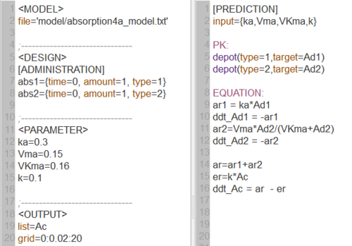
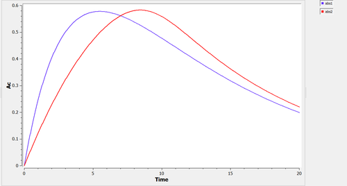
<span style="color:#993300">{{Verbatim|absorption4_script :}}</span> we compute and display the amount in the central compartment when the drug is transferred from the depot to the central compartment with a first-order or saturated (Michaelis-Mentens) absorption process. | <span style="color:#993300">{{Verbatim|absorption4_script :}}</span> we compute and display the amount in the central compartment when the drug is transferred from the depot to the central compartment with a first-order or saturated (Michaelis-Mentens) absorption process. | ||
| Line 95: | Line 92: | ||
| − | + | === Lag-time and transit compartments === | |
<span style="color:#993300">{{Verbatim|absorption5_script :}}</span> we compute and display the amount in the central compartment when a lag time or a transit compartment model is used. | <span style="color:#993300">{{Verbatim|absorption5_script :}}</span> we compute and display the amount in the central compartment when a lag time or a transit compartment model is used. | ||
| Line 102: | Line 99: | ||
| + | <div style="overflow-x:auto"> | ||
{| cellspacing="5" cellpadding="5" | {| cellspacing="5" cellpadding="5" | ||
|style="width:50%"| | |style="width:50%"| | ||
| Line 107: | Line 105: | ||
|style="width:50%"| | |style="width:50%"| | ||
[[File:FirstOrder5_plot.png|400px]] | [[File:FirstOrder5_plot.png|400px]] | ||
| − | |} | + | |} </div> |
See the [[ Explore and visualize PK models with MLXPlore - Part II | Part II]] for the corresponding amounts in the depot compartment and the related $\mlxplore$ project. | See the [[ Explore and visualize PK models with MLXPlore - Part II | Part II]] for the corresponding amounts in the depot compartment and the related $\mlxplore$ project. | ||
| − | + | <br> | |
| − | + | === Summary === | |
<span style="color:#993300">{{Verbatim|absorption6a_script :}}</span> we compute and display the amount in the central compartment for all of the different absorption models presented in the previous examples. | <span style="color:#993300">{{Verbatim|absorption6a_script :}}</span> we compute and display the amount in the central compartment for all of the different absorption models presented in the previous examples. | ||
| Line 119: | Line 117: | ||
| + | <div style="overflow-x:auto"> | ||
{| cellspacing="5" cellpadding="5" | {| cellspacing="5" cellpadding="5" | ||
|style="width:50%"| | |style="width:50%"| | ||
| − | [[File:FirstOrder6.png| | + | [[File:FirstOrder6.png|500px]] |
|style="width:50%"| | |style="width:50%"| | ||
| − | [[File:FirstOrder6_plot.png| | + | [[File:FirstOrder6_plot.png|500px]] |
| − | |} | + | |} </div> |
See the [[ Explore and visualize PK models with MLXPlore - Part II | Part II]] for the corresponding amounts in the depot compartment and the related $\mlxplore$ project. | See the [[ Explore and visualize PK models with MLXPlore - Part II | Part II]] for the corresponding amounts in the depot compartment and the related $\mlxplore$ project. | ||
| + | |||
| + | |||
| + | <br> | ||
| + | == Distribution == | ||
| + | |||
| + | <br> | ||
| + | === One, two and three compartment models === | ||
| + | |||
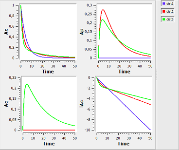
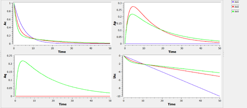
| + | <span style="color:#993300">{{Verbatim|distribution1_script :}}</span> we compute and display the amount in the central and peripheral compartments when the drug is distributed assuming one, two or three compartment models. | ||
| + | Here, $Ap$ and $Aq$ are the amounts in the first and second peripheral compartments and $lAc$ the log-amount in the central compartment. | ||
| + | |||
| + | <div style="overflow-x:auto"> | ||
| + | {| cellspacing="5" cellpadding="5" | ||
| + | |style="width:50%"| | ||
| + | [[File:Distribution1.png|500px]] | ||
| + | |style="width:50%"| | ||
| + | [[File:Distribution1_plot.png|500px]] | ||
| + | |} </div> | ||
| + | |||
| + | |||
| + | <br> | ||
| + | == Elimination == | ||
| + | |||
| + | <br> | ||
| + | === Linear, nonlinear and combined elimination === | ||
| + | |||
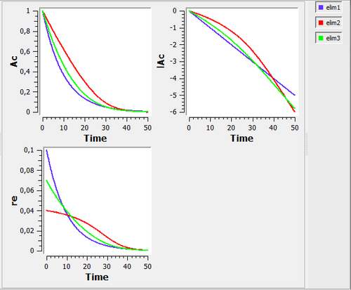
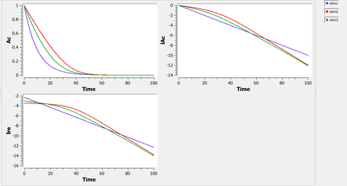
| + | elimination1_script: we compute and display the amount in the central compartment and the rate of elimination when the drug is eliminated with a linear, nonlinear (Michaelis-Mentens) or combined elimination process (linear when $\alpha=1$ and Michaelis-Mentens when $\alpha=1$). | ||
| + | |||
| + | Here, $lAc$ is the log-amount in the central compartment and lre the log-rate of elimination of the drug. By definition, lre is a linear function of time for a linear elimination process. | ||
| + | |||
| + | |||
| + | <div style="overflow-x:auto"> | ||
| + | {| cellspacing="5" cellpadding="5" | ||
| + | |style="width:50%"| | ||
| + | [[File:Elimination1.png|500px]] | ||
| + | |style="width:50%"| | ||
| + | [[File:Elimination1_plot.png|500px]] | ||
| + | |} </div> | ||
Revision as of 12:11, 27 May 2013
Introduction
This is an introductory tutorial for describing and visualizing simple and more complex pharmacokinetic (PK) models.
We will present several PK model examples and visualize the processes of absorption, distribution and elimination that characterize them.
We will suppose in all these examples that a single dose is administered at time t=0. In each example, the modeling goal is defined. Then, the model and requests for graphical outputs are coded in MLXPlore, a new graphical and interactive software for the exploration and visualization of complex pharmacometric models. MLXPlore uses the easy and intuitive MLXtran model coding language, popularized by the Monolix software.
MLXPlore is used here for computing the predicted amount in the central compartment. We further display in [[ Explore and visualize PK models with $\mlxplore$ - Part II | Part II]] the predicted amount in the depot compartment and the MLXPlore project that was used for computing it.
Absorption
First-order and zero-order absorption
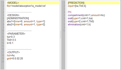
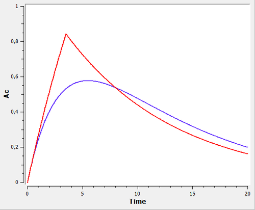
absorption1a_script : this computes and displays the amount (Ac) in the central compartment when the drug is absorbed with a first-order or zero-order absorption process.
Left: In the right-hand side window, the two (first-order and zero-order) models are described using the MLXtran coding language. In the left-hand side window, the structural model, experimental design, parameters and requested graphical output are defined.
Right: The graphical output of MLXPlore, which was told to output the amount Ac in the central compartment with respect to time for zero-order (red) and first-order (blue) absorption.
See the Part II for the corresponding amounts in the depot compartment and the related $\mlxplore$ project.
First-order, zero-order and $\alpha$-order absorption
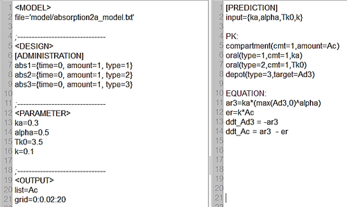
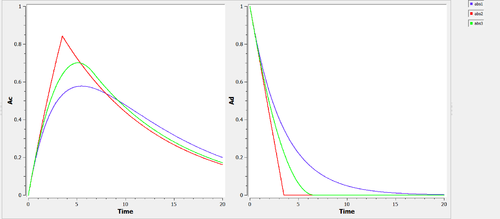
absorption2a_script : we compute and display the amounts in the central and depot compartments when the drug is transferred from the depot to the central compartment with a first-order, zero-order or $\alpha$-order absorption process.
Note $\dot{A}d(t) \, = \, -ka \, Ad^{\alpha}(t).$ Zero-order absorption is obtained with $\alpha=0$ and first-order absorption with $\alpha=1$. The grren curves are with respect to the -\alpha|-order absorption process.
See the Part II for the corresponding amounts in the depot compartment and the related $\mlxplore$ project.
First-order, zero-order and sequential zero-order/first-order absorption
absorption3a_script : we compute and display the amount in the central compartment when the drug is transferred from the depot to the central compartment with a first-order, zero-order or sequential zero-order/first-order absorption process. Here, $r0$ is the absorption rate for the zero-order process and $F0$ the fraction of the dose absorbed in a zero-order process. The green curves refer to the sequential zero-order/first-order absorption process.
See the Part II for the corresponding amounts in the depot compartment and the related $\mlxplore$ project.
First-order and saturated absorption
absorption4_script : we compute and display the amount in the central compartment when the drug is transferred from the depot to the central compartment with a first-order or saturated (Michaelis-Mentens) absorption process. The red curve is now for the saturated absorption process.
See the Part II for the corresponding amounts in the depot compartment and the related $\mlxplore$ project.
Lag-time and transit compartments
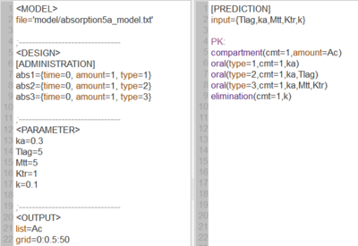
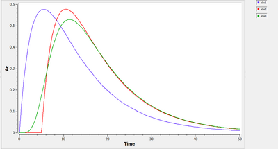
absorption5_script : we compute and display the amount in the central compartment when a lag time or a transit compartment model is used.
Here, the blue curve is for first-order absorption without lag-time, the red curve for the lag-time model and the green one for the transit compartment model. The number of transit compartments is Ntr=Mtt/Ktr. When Mtt=Tlag, the transit compartment model can be seen as a smooth version of the lag-time model. It converges to the lag-time model when the number of compartments increases (i.e., when the transfer rate constant Ktr increases).
See the Part II for the corresponding amounts in the depot compartment and the related $\mlxplore$ project.
Summary
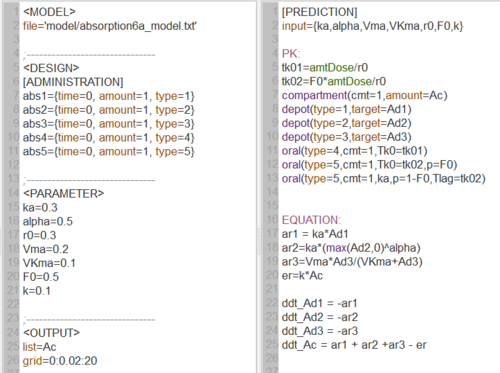
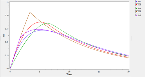
absorption6a_script : we compute and display the amount in the central compartment for all of the different absorption models presented in the previous examples.
In the figure, abs1 is first-order absorption, abs2 is $\alpha$-order absorption, abs3 is saturated absorption, abs4 is zero-order absorption and abs5 is sequential zero-order/first-order absorption.
See the Part II for the corresponding amounts in the depot compartment and the related $\mlxplore$ project.
Distribution
One, two and three compartment models
distribution1_script : we compute and display the amount in the central and peripheral compartments when the drug is distributed assuming one, two or three compartment models. Here, $Ap$ and $Aq$ are the amounts in the first and second peripheral compartments and $lAc$ the log-amount in the central compartment.
Elimination
Linear, nonlinear and combined elimination
elimination1_script: we compute and display the amount in the central compartment and the rate of elimination when the drug is eliminated with a linear, nonlinear (Michaelis-Mentens) or combined elimination process (linear when $\alpha=1$ and Michaelis-Mentens when $\alpha=1$).
Here, $lAc$ is the log-amount in the central compartment and lre the log-rate of elimination of the drug. By definition, lre is a linear function of time for a linear elimination process.
